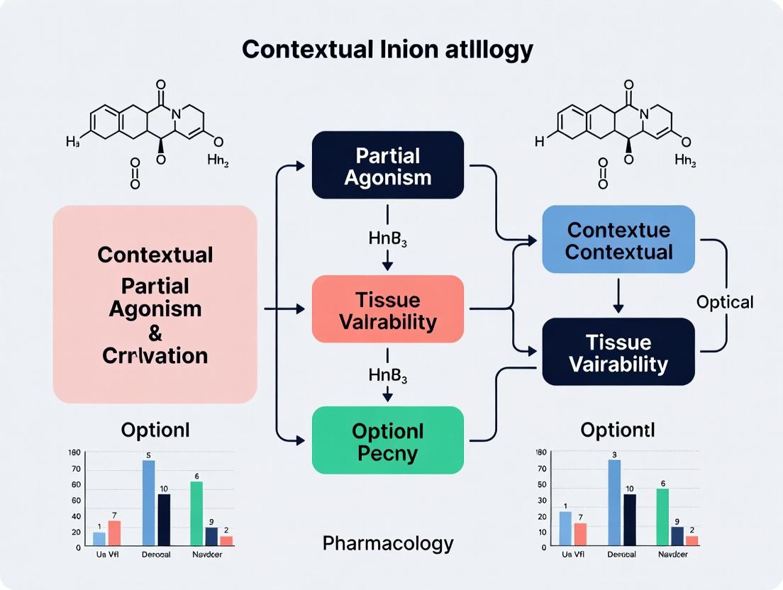
Decoding Contextual Partial Agonism: Unraveling Tissue-Specific Variability in Drug Response for Targeted Therapeutics

Abstract

This article provides a comprehensive examination of contextual partial agonism and its critical dependence on tissue-specific environments. Aimed at researchers, scientists, and drug development professionals, it explores the foundational molecular mechanisms—including receptor density, signaling bias, and allosteric modulation—that drive variability in agonist efficacy. We then detail cutting-edge methodological approaches for quantifying this phenomenon in vitro and in vivo, followed by strategies for troubleshooting and optimizing drug candidates plagued by unpredictable tissue responses. Finally, the article covers rigorous validation frameworks and comparative analyses against full agonists and antagonists. The synthesis offers a roadmap for harnessing tissue variability to design safer, more precise therapeutics with minimized off-target effects.

Understanding the Roots: Core Mechanisms of Contextual Partial Agonism and Tissue-Specific Signaling

In pharmacology, Contextual Partial Agonism (CPA) is the phenomenon where a ligand exhibits varying degrees of partial agonism—producing a submaximal response relative to a full agonist—depending on the specific cellular or tissue context. This variability arises from differences in cellular signaling components, such as receptor density, G-protein/GEF expression ratios, effector coupling efficiency, and the presence of regulatory proteins (e.g., β-arrestins, RGS proteins). CPA complicates drug development by making in vitro-to-in-vivo and inter-tissue predictions unreliable. This technical support center provides resources for troubleshooting CPA research within the thesis framework of "Addressing Contextual Partial Agonism Tissue Variability."

FAQs & Troubleshooting Guides

Q1: Our lead compound shows 60% efficacy in Cell Line A but only 25% in primary Tissue B. Is this CPA? A: Likely yes. First, confirm receptor expression levels. Use quantitative methods (e.g., radioligand binding, flow cytometry) to measure receptor density (B_max). High receptor reserve in one system can mask partial agonism, making a ligand appear more efficacious.

• Troubleshooting Steps:
  • Measure Receptor Density: Perform saturation binding assays on membranes from both systems.
  • Normalize Response: Plot response as a function of receptor occupancy. CPA is indicated if the occupancy-response curves differ between systems.
  • Check Effector Coupling: Assess downstream signaling markers (e.g., cAMP, IP1, pERK) to identify pathway-specific bias or inefficiency.

Q2: How do we differentiate CPA from biased agonism? A: Biased agonism refers to preferential activation of one signaling pathway over another by a ligand within the same cellular system. CPA refers to changes in the degree of efficacy for a given pathway across different systems. They are often interconnected.

• Experiment: Perform a Pathway Potency/Efficacy Ratio experiment in multiple cell types.

Cell/Tissue Type	Pathway 1 (e.g., G-protein) EC₅₀	Pathway 1 E_max (%)	Pathway 2 (e.g., β-arrestin) EC₅₀	Pathway 2 E_max (%)	ΔEmax (Path1-Path2)
Recombinant Cell Line	10 nM	100%	50 nM	80%	+20%
Primary Cell Type A	15 nM	75%	45 nM	90%	-15%
Primary Tissue B	12 nM	40%	200 nM	30%	+10%

A consistent ligand bias profile (similar ΔEmax) with varying absolute efficacies (E_max) points to CPA. A shifting ΔEmax indicates the bias itself is context-dependent.

Q3: Our in vivo efficacy does not match optimized in vitro profiles. How to model CPA? A: Single-pathway in vitro models fail to capture tissue context. Implement a Multi-Parameter Signaling Assay in a relevant primary cell or native tissue system.

• Protocol: Simultaneous Monitoring of G-protein and β-arrestin Signaling.
  • Cell System: Use primary cells or a cell line transfected with a GPCR fused to a BRET-based biosensor (e.g., Gα-Rluc8 with GFP-tagged effector; β-arrestin-Rluc8 with GFP-tagged GPCR).
  • Stimulation: Treat cells with a full agonist, your partial agonist, and antagonist control.
  • Measurement: Record BRET signals in real-time using a plate reader.
  • Analysis: Generate time-course and concentration-response data for both pathways from the same cell population. Compare the relative efficacy (E_max) and potency (EC₅₀) ratios across different primary cell isolates.

Experimental Protocol: Determining Contextual Agonism Parameters

Title: Quantifying CPA Using an Operational Model of Agonism. Objective: To derive system-independent parameters (transduction coefficient, log(τ/Κ_A)) for a partial agonist across two tissue contexts.

Materials:

• Tissue/cell preparations from two distinct organ sources expressing the target receptor.
• Test partial agonist, reference full agonist, and neutral antagonist.
• Equipment for functional response measurement (e.g., cAMP, calcium flux, tissue myography).

Method:

• Generate Agonist Concentration-Response Curves (CRCs): For both the full and partial agonist in each tissue system. Normalize response to the system maximum (full agonist in that tissue).
• Generate Antagonist Schild Plot: Use a neutral antagonist in each system to determine the agonist dissociation constant (Κ_A) for the partial agonist.
• Fit Data to Operational Model: Fit the CRC data to the Black/Leff operational model using nonlinear regression: Response = (Em * τ^n * [A]^n) / ( (ΚA + [A])^n + τ^n * [A]^n ).
  • Em = System maximum response.
  • [A] = Agonist concentration.
  • ΚA = Agonist-receptor dissociation constant (from Schild analysis).
  • τ = Transducer constant (measure of coupling efficiency).
  • n = Slope factor.
• Calculate log(τ/ΚA): This is the system-independent transduction coefficient. A constant log(τ/ΚA) for the agonist across tissues suggests the observed CPA is due to system differences (τ), not ligand properties.

Visualizations

Diagram 1: CPA Arises from System Variables

Diagram 2: Operational Model Analysis Workflow

The Scientist's Toolkit: Key Research Reagent Solutions

Item	Function in CPA Research
Pathway-Selective Biosensors (e.g., cAMP GloSensor, BRET-based G-protein/β-arrestin sensors)	Enable real-time, simultaneous quantification of multiple signaling pathways from the same cell population to dissect bias and efficacy.
Receptor Density Quantification Kit (e.g., fluorescent/radiolabeled antagonist, anti-receptor Ab with QIF standards)	Accurately measure B_max, a critical variable for interpreting efficacy differences between tissues.
Operational Model Fitting Software (e.g., GraphPad Prism with specific equations, custom R/Python scripts)	Essential for deriving system-independent ligand parameters (log(τ/Κ_A)) from functional data.
Native/Relevant Cell Systems (Primary cells, patient-derived cells, organoids)	Provide the necessary physiological "context" with native expression levels of receptors, effectors, and regulators.
Universal Reference Agonist & Antagonist (Well-characterized full agonist and neutral antagonist for the target)	Critical internal controls for normalizing responses and determining K_A across different experimental systems.

Troubleshooting Guide & FAQs

Q1: Our lead partial agonist candidate shows excellent efficacy in cardiac tissue assays but fails in neuronal tissue models. What are the primary factors to investigate? A: This is a classic manifestation of Contextual Partial Agonism. Key factors to investigate, in order of priority, are:

• Receptor Expression Density: The same receptor (e.g., β2-adrenergic) is often expressed at vastly different levels across tissues. Partial agonists are highly sensitive to this "receptor reserve."
• Signalosome Composition: Investigate the presence or absence of key effector proteins (e.g., specific G-protein subtypes, β-arrestin isoforms, kinases like GRKs) that form unique signaling complexes in different tissues.
• Coupling Efficiency: The efficiency with which an occupied receptor activates downstream G-proteins differs between tissue systems.

Q2: How can we experimentally quantify receptor density (Bmax) and ligand affinity (Kd) in our different target tissues? A: Perform a Saturation Binding Assay using a radiolabeled or fluorescent high-affinity antagonist.

Protocol: Saturation Binding for Tissue Homogenates

• Tissue Preparation: Homogenize snap-frozen cardiac and neuronal tissue samples separately in ice-cold buffer. Centrifuge to isolate membrane fractions.
• Incubation: Incubate a constant amount of membrane protein with increasing concentrations of the labeled ligand ([L]) in duplicate or triplicate. Include parallel wells with a 1000-fold excess of unlabeled competitor to define non-specific binding (NSB).
• Separation & Measurement: Filter the samples to separate bound from free ligand. Measure the bound radioactivity/fluorescence.
• Data Analysis: Calculate specific binding (Total Binding – NSB). Plot Specific Bound (y) vs. [L] (x). Fit data to a one-site binding model: B = (Bmax * [L]) / (Kd + [L]) Bmax (total receptor density) and Kd (equilibrium dissociation constant) are derived from the curve fit.

Q3: Our data suggests differential G-protein coupling. What's the best method to profile this? A: Utilize a GTPγS ([³⁵S]Guanosine-5′-O-(3-thiotriphosphate)) Binding Assay. It directly measures receptor-mediated G-protein activation.

Protocol: GTPγS Binding Assay

• Membrane Incubation: Incubate tissue membranes with GDP (to stabilize G-proteins) and varying concentrations of your partial agonist.
• Initiation: Add [³⁵S]GTPγS (non-hydrolyzable GTP analog). The agonist-stimulated receptor promotes GDP/GTPγS exchange on the Gα subunit.
• Measurement: Terminate reaction by filtration. Bound radioactivity correlates with activated G-proteins.
• Analysis: Plot % stimulation over basal vs. agonist concentration. The Emax indicates coupling efficacy, and EC50 indicates potency in that tissue system.

Q4: How do we integrate these data to predict in vivo tissue variability? A: Construct a Quantitative Systems Pharmacology (QSP) model. Input your experimental parameters to simulate tissue response.

Table 1: Saturation Binding Parameters for Target Tissues

Tissue Type	Bmax (fmol/mg protein)	Kd (nM)	Key Receptor Isoform
Cardiac	125.4 ± 15.2	0.85 ± 0.12	β1-AR (80%), β2-AR (20%)
Neuronal	32.1 ± 5.6	0.92 ± 0.18	β2-AR (95%)
Hepatic	58.7 ± 8.3	1.10 ± 0.21	β2-AR (100%)

Table 2: Functional Response (GTPγS) to Partial Agonist 'X'

Tissue Type	Basal Activity (cpm)	Max Stimulation (% over Basal)	EC50 (nM)	Intrinsic Relative Activity (%)*
Cardiac	550 ± 45	245 ± 18%	15.2	85
Neuronal	310 ± 32	62 ± 8%	18.5	22
Hepatic	480 ± 40	180 ± 15%	22.7	65

*Normalized to a full reference agonist in each tissue.

Visualizations

Tissue-Specific Signaling Determinants

Tissue Variability Investigation Workflow

The Scientist's Toolkit: Research Reagent Solutions

Reagent / Material	Function in Investigation	Key Consideration
Tissue Membrane Preparations	Source of native receptors and signaling machinery.	Maintain consistency in protein concentration and freeze-thaw cycles.
[³H]-Dihydroalprenolol (DHA)	Radiolabeled antagonist for β-adrenergic receptor saturation binding.	High specific activity required for low Bmax tissues.
[³⁵S]GTPγS	Radiolabeled non-hydrolyzable GTP analog for G-protein activation assays.	Requires GDP in assay buffer to suppress basal activity.
GRK/Arrestin Isoform-Selective Antibodies	Detect tissue-specific expression of signaling regulators via immunoblot.	Validate antibody specificity for the target isoform.
QSP Modeling Software (e.g., R, MATLAB with SimBiology)	Integrates binding/functional data to predict tissue-level pharmacology.	Model must account for system-specific coupling parameters.
Reference Full Agonist & Inverse Agonist	Critical controls for defining system's maximal response and basal tone.	Use well-characterized ligands (e.g., Isoprenaline, ICI-118,551 for β-AR).

Troubleshooting Guide & FAQs

Q1: My functional assay in HEK293 cells shows a potent, full agonist response to Compound X. However, in a primary tissue assay, the same compound acts as a low-efficacy partial agonist. Is this a receptor reserve issue? A1: Very likely. The high recombinant receptor expression in HEK293 cells creates a large receptor reserve, allowing even low-efficacy agonists to produce a maximal system response. Primary tissues typically have lower, physiological receptor density, revealing the true low intrinsic efficacy of the compound. Troubleshooting Steps:

• Perform a radioligand binding assay to quantify receptor density (Bmax) in both cell systems.
• Conduct concentration-response curves in the HEK293 line after irreversible receptor inactivation (e.g., with alkylating agents like phenoxybenzamine) to progressively reduce the receptor reserve. You should observe a shift from a full to a partial agonist profile.

Q2: How can I experimentally quantify and compare "spare receptors" between two different tissue types? A2: The operational measure is the "Transduction Coefficient" (τ/KA ratio). A higher τ indicates a greater signaling capacity/receptor reserve. Experimental Protocol:

• Generate Agonist Concentration-Response Curves: For a full agonist, in both Tissue A and Tissue B.
• Irreversibly Inactivate a Fraction of Receptors: Treat tissues with an alkylating agent to reduce functional receptor density.
• Re-run Concentration-Response Curves: Observe the rightward shift in the EC50.
• Analyze Data via Operational Model Fitting: Fit the data to the Black/Leff Operational Model (using software like Prism) to estimate the parameters:
  • [Agonist]: Concentration.
  • E: Effect.
  • Em: Maximum system response.
  • τ: Transduction coefficient (a measure of efficiency).
  • KA: Equilibrium dissociation constant.
  • n: Slope factor.
• Compare τ values: A tissue with a higher τ has a greater receptor reserve for that agonist.

Q3: My model predicts spare receptors, but my β-arrestin recruitment assay shows no signal amplification compared to G-protein signaling. Why? A3: Receptor reserve is pathway-specific. Traditional "spare receptors" often refer to highly amplified pathways like G-protein-coupled second messenger systems (e.g., cAMP, IP3). β-arrestin recruitment may have a linear or less efficient coupling with minimal reserve. This highlights contextual partial agonism—a ligand may be a full agonist for Pathway A (with reserve) but a partial agonist for Pathway B (no reserve) in the same cell. Troubleshooting: Repeat the operational analysis (Q2) separately for each signaling pathway output.

Data Tables

Table 1: Example Receptor Density (Bmax) & Operational Parameters in Different Tissues

Tissue / Cell Type	Receptor (Target)	Bmax (fmol/mg protein)	Full Agonist (Emax %)	τ (Gq-IP3 pathway)	KA (nM)	Inferred Receptor Reserve
Recombinant HEK293	β2-Adrenoceptor	1500 ± 210	100%	12.5	5.2	High
Cardiac Myocyte	β2-Adrenoceptor	85 ± 15	100%	2.1	4.8	Low
Vascular Smooth Muscle	α1-Adrenoceptor	45 ± 8	100%	15.3	1.5	High
Recombinant CHO	Muscarinic M3	2200 ± 350	100%	8.7	3.0	High

Table 2: Impact of Receptor Alkylation on Agonist Profile (Theoretical Data)

Treatment (Receptor Density)	Compound Y (Intrinsic Efficacy = 0.3)
	EC50 (nM)	Emax (% System Max)
Native HEK293 (Bmax = 1000)	1.1	100% (Full Agonist)
Post-Alkylation (Bmax ~ 100)	12.5	45% (Partial Agonist)
Post-Alkylation (Bmax ~ 20)	55.0	15% (Weak Partial Agonist)

Detailed Experimental Protocols

Protocol 1: Quantifying Receptor Density (Bmax) via *Saturation Radioligand Binding.* Objective: Determine total receptor number in a cell or tissue membrane preparation. Materials: See "Scientist's Toolkit" below. Method:

• Prepare membrane homogenates from tissue/cells. Determine protein concentration.
• In a 96-well plate, incubate a constant amount of membrane protein with increasing concentrations of the radiolabeled antagonist (e.g., [³H]N-methylscopolamine for muscarinic receptors). Include wells for total binding and non-specific binding (NSB) defined by a high concentration of unlabeled competitor (e.g., 1 μM atropine).
• Incubate to equilibrium (e.g., 60-90 mins at 25°C).
• Terminate reaction by rapid filtration through GF/C filter plates using a cell harvester. Wash filters to remove unbound ligand.
• Dry filters, add scintillation cocktail, and count radioactivity.
• Analysis: Subtract NSB from total binding at each point to get specific binding. Fit specific binding data to a one-site saturation binding model: B = (Bmax * [L]) / (KD + [L]), where B is bound, [L] is free ligand concentration. Bmax (receptor density) and KD (affinity) are derived.

Protocol 2: Irreversible Receptor Inactivation to Assess Receptor Reserve. Objective: To reduce functional receptor density and reveal intrinsic efficacy. Materials: Alkylating agent (e.g., Phenoxybenzamine HCl), appropriate vehicle control, functional assay buffer. Method:

• Prepare tissue strips or cell suspensions. Divide into groups.
• Treatment: Incubate test groups with a single concentration of phenoxybenzamine (e.g., 1-10 μM for 10-30 minutes) sufficient to inactivate 70-90% of receptors. Include a vehicle-only control group.
• Wash: Perform extensive, vigorous washing (e.g., 6 x 10 mins in large volume buffer) to remove all unbound alkylating agent.
• Functional Assay: Construct concentration-response curves for the agonist of interest in both alkylated and control tissues.
• Analysis: Fit data to the operational model. The alkylated tissue will have a greatly reduced τ value. The shift in the agonist's profile directly demonstrates the role of spare receptors.

Pathway & Workflow Diagrams

Diagram 1: G-Protein Signal Amplification Cascade

Diagram 2: Experimental Workflow to Quantify Receptor Reserve

The Scientist's Toolkit: Key Research Reagent Solutions

Item	Function in Receptor Reserve Studies
[*³H]-Labeled Antagonists (e.g., [³H]CGP-12177 for β-AR)	High-affinity radioligands for saturation binding experiments to determine receptor density (Bmax).
Irreversible Antagonists (e.g., Phenoxybenzamine, EEDQ)	Covalently binds to and inactivates a population of receptors, allowing experimental reduction of receptor density.
Cell Membrane Preparation Kits	For consistent isolation of membrane proteins from tissues or cultured cells for binding assays.
GF/C Filter Plates & Harvester	Essential for rapid separation of bound from free radioligand in high-throughput binding assays.
Software with Operational Model (e.g., GraphPad Prism)	Contains built-in equations (e.g., "Operational model of agonism") to fit functional data and derive τ and KA.
Pathway-Specific Assay Kits (e.g., cAMP, IP3, β-Arrestin BRET)	To measure agonist output across different signaling pathways and assess pathway-specific receptor reserve.

Troubleshooting Guides & FAQs

Q1: Our biased ligand shows the expected G protein bias in a cell-based cAMP assay, but no β-arrestin recruitment is detected in the Tango assay. What could be wrong?

A: This discrepancy often stems from assay system configurations.

• Troubleshooting Steps:
  • Receptor Expression Level: The Tango assay requires the engineered receptor (fused to a transcription factor) to be expressed at optimal levels. Check transfection efficiency and receptor density via flow cytometry or a surface ELISA.
  • Promoter/Readout Sensitivity: Ensure the inducible promoter driving the reporter gene (e.g., luciferase) is highly sensitive and the substrate is fresh. Compare against a positive control ligand known to recruit β-arrestin in your system.
  • Time Course: β-arrestin-dependent transcription is slower. Extend the incubation time with your ligand (e.g., 6-24 hours) versus the rapid G protein cAMP response (minutes).
  • Ligand Stability: Confirm ligand stability over the longer Tango assay duration.

Q2: We observe significant tissue-to-tissue variability in bias factors for the same GPCR ligand. Is this an artifact?

A: Not necessarily; it's a core aspect of contextual partial agonism. Variability can arise from:

• Endogenous Expression Profiles: Different tissues express varying levels of G protein subtypes, GRKs, β-arrestins, and regulatory proteins (e.g., RGS proteins).
• Signalosome Context: The cellular background (e.g., HEK293 vs. primary neurons) dictates available signaling partners.
• Troubleshooting/Action:
  • Characterize and report the exact cellular context (cell line, passage, receptor expression level in fmol/mg).
  • Measure and compare the system bias of your assay platforms using a standard unbiased agonist (e.g., full natural agonist) as a reference point. Use the Black-Leff operational model to calculate ΔΔlog(τ/KA) or ΔΔlog(Emax/EC50) values.

Q3: How do we validate that observed bias is genuine and not due to assay artifacts like signal amplification or ceiling effects?

A: Employ rigorous pharmacological validation.

• Method:
  • Full Concentration-Response Curves: Always run full curves (e.g., 10-12 point) for each pathway. Do not rely on single-point data.
  • Reference Agonists: Include a balanced reference agonist (e.g., the endogenous ligand) in every experiment to define "unbiased" in your specific system.
  • Operational Modeling: Fit data to the Black-Leff operational model to calculate transducer ratios (τ/KA) for each ligand in each pathway. The bias factor is ΔΔlog(τ/KA).
  • Pathway-Specific Inhibition: Use selective inhibitors to confirm pathway identity (e.g., Pertussis toxin for Gi/o; BRET-based β-arrestin mutants; CRISPR knockout of β-arrestin 1/2).

Data Presentation: Comparative Analysis of Bias Quantification Methods

Method	Measured Output	Typical Assay Format	Key Advantage	Key Limitation	Suited for Contextual Variability Research?
ΔΔLog(τ/KA)	Transducer Coefficient Ratio	BRET/FRET cAMP, ERK phosphorylation, β-arrestin recruitment (any full curve)	Most rigorous; accounts for efficacy & affinity; system-independent.	Requires robust curve fitting & modeling expertise.	Yes - Gold standard for cross-tissue comparison.
ΔΔLog(Emax/EC50)	Empirical Efficacy/Potency Ratio	Calcium flux, IP-1 accumulation, SNAP-tag internalization.	Simpler to calculate from experimental data.	Can conflate system bias with ligand bias if pathways have different amplification.	With caution - Must be normalized to reference agonist in each system.
*Bias Plot (Log(τ/KA)) *	Relative Agonist Activity	Any two pathways with full curve data.	Visual, intuitive representation of bias relative to a reference point.	Qualitative to semi-quantitative.	Yes - Excellent for visualizing shifts across tissues.
Pathway-Specific BRET/FRET	Real-time protein interaction	Live-cell BRET (e.g., Gαβγ dissociation, β-arrestin recruitment).	Provides kinetic data on early signaling events.	Requires specialized biosensors & equipment.	Yes - Reveals kinetic bias differences in native contexts.

Experimental Protocols

Protocol 1: Quantifying G Protein Bias via cAMP Inhibition Assay (Gi/o-coupled GPCR) Objective: Measure ligand efficacy/potency for the Gi/o pathway via inhibition of forskolin-stimulated cAMP.

• Cell Preparation: Seed cells stably expressing the target GPCR into a 96-well white assay plate.
• Stimulation: Pre-incubate cells with a range of ligand concentrations (11-point, 1:3 serial dilution) for 15 min. Then add forskolin (at EC80 concentration) for 30 min at 37°C.
• cAMP Detection: Lyse cells and quantify cAMP using a HTRF (Cisbio) or AlphaLISA (PerkinElmer) kit according to manufacturer instructions. Include a cAMP standard curve.
• Data Analysis: Normalize data to forskolin response alone (0% inhibition) and buffer control (100% inhibition). Fit normalized concentration-response curves using a 4-parameter logistic (4PL) model in GraphPad Prism. Calculate Emax and EC50.
• Bias Calculation: Perform steps 1-4 in parallel for a β-arrestin recruitment assay (see Protocol 2). Calculate bias factors using the operational model (see FAQ A3).

Protocol 2: Quantifying β-Arrestin Bias via NanoBiT Complementation Assay Objective: Measure ligand-induced β-arrestin2 recruitment to the GPCR.

• Biosensor Transfection: Co-transfect cells with:
  • A plasmid encoding the target GPCR C-terminally tagged with LgBiT.
  • A plasmid encoding β-arrestin2 N-terminally tagged with SmBiT.
  • (Optional: A transfection control plasmid).
• Cell Preparation: 24h post-transfection, seed cells into a 96-well white assay plate.
• Reconstitution & Reading: Following manufacturer (Promega) guidelines, add the cell-permeable LgBiT substrate (furimazine). Immediately read baseline luminescence on a plate reader.
• Stimulation: Add a range of ligand concentrations (same as Protocol 1) and monitor real-time luminescence for 30-60 minutes.
• Data Analysis: Calculate ΔRLU (peak luminescence - baseline). Fit ΔRLU vs. log[ligand] curves using a 4PL model. Calculate Emax and EC50 for bias calculation relative to G protein pathway data.

Visualization: Signaling Pathway & Workflow Diagrams

Title: GPCR Signaling Bias Pathways

Title: Bias Factor Determination Workflow

The Scientist's Toolkit: Research Reagent Solutions

Item	Function/Application in Bias Research	Example/Notes
Path-Specific Biosensors	Live-cell, real-time monitoring of discrete signaling events (G protein activation, β-arrestin recruitment).	cAMP: GloSensor (Promega). β-arrestin: NanoBiT (Promega), Tango (Invitrogen). Kinases: ERK, AKT TR-FRET kits (Cisbio).
Operational Modeling Software	Pharmacological data fitting to calculate unbiased transducer coefficients (τ/KA) and bias factors.	GraphPad Prism (with Black-Leff plug-in), Bias Calculator (from Roth/Lefkowitz labs).
Reference Agonists	Critical benchmark to define "unbiased" signaling in any given cellular system.	Endogenous full agonist (e.g., Isoproterenol for β2AR). System-balanced synthetic agonist (must be characterized in literature).
Pathway-Selective Inhibitors	To confirm the identity of the measured signaling pathway and probe context.	G Protein: Pertussis Toxin (Gi/o), NF023 (Gq). β-Arrestin: CRISPR knockout, dominant-negative mutants. GRKs: siRNA knockdown panels.
Contextual Cell Models	To study tissue variability and partial agonism context.	Recombinant lines (varying G protein/GRK expression). Primary cells (from relevant tissues). iPSC-derived cells (disease-relevant contexts).
Tagged Receptor Constructs	For biosensor assays and localization studies.	SNAP-tag, HALO-tag, LgBiT/SmBiT. Ensure tagging does not alter receptor pharmacology.

Troubleshooting Guides & FAQs

FAQ 1: Why do I observe high constitutive activity in my assay when expressing a receptor of interest, even in the absence of agonist?

• Answer: High basal signaling is frequently linked to receptor overexpression, which can lead to promiscuous coupling to available G proteins or β-arrestins beyond physiological levels. It can also indicate a high level of endogenous G protein/effector expression in your chosen cellular background. To troubleshoot:
  • Titrate your receptor transfection DNA to find the lowest expression level yielding a robust signal-to-noise window.
  • Use a cell line with lower endogenous G protein expression (e.g., CHO-K1 vs. HEK-293).
  • Include a constitutive activity control (e.g., empty vector, vector expressing an unrelated GPCR).

FAQ 2: My candidate compound acts as a full agonist in Cell Line A but shows only partial agonism in Cell Line B. Is the compound or my assay faulty?

• Answer: This is a classic manifestation of "contextual partial agonism" tied to Cellular Background. The discrepancy is likely valid and arises from differences in effector or coupling protein expression (e.g., Gα subtype ratios, GRK levels, β-arrestin pools) between the two lines. The compound's efficacy is not absolute but depends on the signaling capacity of the cell.

FAQ 3: How can I systematically quantify the differences in effector protein expression across my panel of cell models?

• Answer: Implement a quantitative proteomics approach (e.g., Targeted Mass Spectrometry, LC-MS/MS) or high-quality quantitative immunoblotting.
  • Protocol: Perform cell lysis, quantify total protein, load equal masses, and run SDS-PAGE. Use a multiplexed fluorescent Western blot system with validated, target-specific antibodies against Gα subunits (Gαs, Gαi, Gαq/11, Gα12/13), Gβγ, adenylate cyclase isoforms, GRKs, and β-arrestins 1/2. Normalize signals to a stable endogenous control (e.g., GAPDH, β-actin). Compare relative expression levels across cell lysates run on the same gel.

FAQ 4: My β-arrestin recruitment assay shows no signal, despite confirmed receptor expression. What are the key checks?

• Answer: This suggests a deficiency in the required coupling proteins.
  • Verify Cellular Background: Ensure your host cell line expresses sufficient levels of β-arrestin and the necessary GRKs for your receptor. Some common lines (e.g., certain CHO variants) have very low endogenous β-arrestin. Consider using a β-arrestin-overexpressing line or co-transfecting β-arrestin and a relevant GRK.
  • Positive Control: Test a known β-arrestin-biased agonist or a positive control receptor (e.g., AT1R for angiotensin II) in your system.

FAQ 5: How can I prove that a shift in agonist efficacy profile is directly caused by G protein expression levels?

• Answer: Perform a G protein complementation or reconstitution experiment.
  • Protocol: Use a cell line deficient in a specific Gα subunit (e.g., Gαs-knockout HEK-293). Measure the agonist response (e.g., cAMP accumulation) in the knockout background—it should be absent or minimal. Then, co-transfect the receptor with increasing amounts of the missing Gαs subunit plasmid. Plot agonist efficacy (Emax) against quantified Gαs expression levels (via Western blot). A direct correlation confirms G protein expression as the key determinant.

Table 1: Relative Expression Levels of Key Signaling Proteins in Common Cell Lines

Cell Line	Gαs (fmol/µg)	Gαi (fmol/µg)	Gαq (fmol/µg)	β-arrestin-2 (A.U.)	GRK2 (A.U.)	Common Use
HEK-293	12.5 ± 1.8	18.3 ± 2.1	9.7 ± 1.2	High	High	Broad GPCR screening
CHO-K1	8.2 ± 0.9	15.1 ± 1.5	7.5 ± 0.8	Low	Moderate	cAMP, Ca2+ assays
U2OS	5.1 ± 0.7	9.4 ± 1.1	4.3 ± 0.5	Moderate	Low	β-arrestin recruitment
HTLA Cells	6.5 ± 1.0	10.2 ± 1.3	5.8 ± 0.7	Very High	High	TRUPATH, β-arrestin

Data is representative, compiled from recent literature. A.U. = Arbitrary Units from quantitative Western blot.

Table 2: Impact of Gαs Overexpression on Agonist Efficacy (Emax %) for a β2-Adrenergic Receptor Ligand

Transfected Gαs Plasmid (ng)	Measured Gαs Increase (Fold)	Agonist A (Emax %)	Agonist B (Emax %)
0 (Endogenous)	1.0	100 (Reference)	45
100	2.5 ± 0.3	100	68
250	5.1 ± 0.6	100	89
500	8.8 ± 1.1	100	95

Simulated data illustrating how cellular G protein levels contextualize partial agonism.

Experimental Protocols

Protocol: Quantifying Contextual Agonism via cAMP in Isogenic Lines with Modified Gαs

Objective: To demonstrate that agonist efficacy is a function of cellular Gαs protein expression. Materials: Parental Cell Line, Gαs-KO Cell Line (via CRISPR), Gαs expression plasmid, cAMP BRET or ELISA kit, Receptor of Interest (ROI) plasmid, agonist compounds. Steps:

• Seed Gαs-KO cells in 3 separate plates for transfection.
• Plate 1: Transfect with ROI plasmid only.
• Plate 2: Co-transfect ROI plasmid + Low dose (100ng) Gαs plasmid.
• Plate 3: Co-transfect ROI plasmid + High dose (500ng) Gαs plasmid.
• 48h post-transfection, serum-starve cells for 2-4 hours.
• Stimulate cells with a full concentration-response curve of Agonist A and Agonist B (partial agonist) in assay buffer.
• Lyse cells and quantify cAMP accumulation using a standardized kit.
• In parallel, lyse cells from each condition for quantitative Gαs Western blot analysis.
• Fit cAMP concentration-response data to a sigmoidal curve to determine Emax for each agonist.
• Correlate Emax values with the quantified Gαs expression level for each transfection condition.

Signaling Pathways & Workflows

Diagram Title: Cellular Background Dictates Signaling Output

Diagram Title: Workflow to Link Efficacy to Cellular Background

The Scientist's Toolkit: Research Reagent Solutions

Reagent / Material	Primary Function in This Context
PathHunter or Tango GPCR Cells	Pre-engineered cell lines with uniform, high expression of β-arrestin and enzyme fragments, standardizing that aspect of cellular background.
TRUPATH BRET Biosensor Kits	Comprehensive set of validated G protein biosensors for quantifying specific G protein activation, controlling for expression.
G protein Specific Antibodies (Validated for Quant. WB)	Essential for measuring endogenous levels of Gα subtypes, GRKs, and β-arrestins across cell models.
CRISPR/Cas9 Gene Editing Tools	To create isogenic cell lines knockout or knock-in of specific effector proteins (e.g., Gαs KO, β-arrestin KO).
NanoBRET Target Engagement Kits	To measure real-time binding of ligands to receptors in live cells, independent of signaling bias, controlling for receptor expression.
Membrane-Tethered Gα Subunit Constructs	Engineered G proteins that localize to the membrane, reducing variability caused by differential expression of endogenous G proteins.
SPR or Biacore Systems	For label-free, cell-free assessment of binding kinetics, removing all cellular background variables.

Technical Support Center

Frequently Asked Questions (FAQs)

Q1: When validating a contextual partial agonist in a new tissue model, my phospho-protein assay shows unexpected activation of an off-target pathway (e.g., ERK in a primarily p38-focused assay). What are the primary systems-level causes? A1: This is a classic symptom of network plasticity. In a systems view, your agonist is likely modulating a key hub node (e.g., a shared kinase like SRC or RAF1) with different connectivity in your new tissue context. The differential expression of pathway inhibitors (e.g., DUSPs, phosphatases) or scaffold proteins (e.g., KSR1) reroutes the signal. First, quantify the expression of these modulators in your new tissue versus your standard model (see Table 1). Follow Protocol A to perform a co-immunoprecipitation network integrity check.

Q2: My computational model, built from liver cell line data, fails to predict the partial agonist efficacy in primary cardiac cells. Which parameters should be prioritized for recalibration? A2: The highest-impact parameters are typically those with the highest network centrality in your new tissue-specific protein-protein interaction (PPI) network. Prioritize recalibration of: 1) Receptor coupling efficiency (G-protein/β-arrestin bias ratios), 2) Expression levels of feedback regulators (e.g., RGS proteins, β-arrestins), and 3) Basal activity states of shared effector proteins (see Table 2). Use Protocol B for targeted quantitative proteomics to obtain these values.

Q3: How can I distinguish true tissue-specific network rewiring from simple differences in receptor expression levels? A3: Normalize your response data to receptor number (using a radioligand binding or flow cytometry assay). Then, perform a pathway activation potency shift analysis. If the rank order of pathway activation (e.g., p38 > AKT > ERK in Tissue A vs. AKT > p38 > ERK in Tissue B) changes after normalization, it indicates fundamental network rewiring. If the rank order is preserved but overall efficacy scales with receptor number, the difference is primarily stoichiometric. See Protocol C.

Troubleshooting Guides

Issue: Low correlation between predicted (from network model) and observed dose-response curves for a target pathway. Steps:

• Verify Input Data: Ensure your tissue-specific protein quantification data (e.g., from mass spectrometry) is normalized to total protein, not a single housekeeper.
• Check Feedback Loops: Your model may lack critical tissue-specific negative feedback. Experimentally inhibit candidate feedback nodes (e.g., with siRNA against a specific DUSP) and re-run the dose-response. If the correlation improves, integrate that feedback.
• Audit Edge Logic: Review if interactions in your network are assumed to be always active (static). Replace key edges with condition-dependent (phosphorylation-dependent) logic.

Issue: Inconsistent partial agonism profile (τ value) across different cellular endpoints (e.g., cAMP vs. β-arrestin recruitment) in the same tissue. Steps:

• Test for System Bias: This is expected behavior if the agonist stabilizes a receptor conformation that preferentially engages one signaling partner. Quantify using the Operational Model for each endpoint.
• Assay Temporal Resolution: The two endpoints may have different temporal peaks. Perform a high-resolution time-course experiment (see Protocol D).
• Confirm Receptor Dimerization State: The agonist may alter dimerization with a modulating partner (e.g., another GPCR) that influences one endpoint more than the other. Use a BRET dimerization assay.

Experimental Protocols

Protocol A: Co-Immunoprecipitation for Network Integrity Check Objective: Validate physical interactions in a suspected rewired module.

• Lyse tissue/cells in non-denaturing lysis buffer (containing protease/phosphatase inhibitors).
• Pre-clear lysate with Protein A/G beads for 30 min at 4°C.
• Incubate with antibody against your hub protein (e.g., RAF1) or target receptor overnight at 4°C.
• Add beads for 2 hours. Wash beads 4x with cold lysis buffer.
• Elute proteins in 2X Laemmli buffer. Analyze by western blot for expected and suspected off-target interactors (e.g., MAP3Ks, scaffold proteins).

Protocol B: Targeted Proteomics for Key Network Parameters Objective: Quantify absolute abundance of key signaling proteins.

• Prepare tissue/cell lysates in RIPA buffer. Quantify total protein.
• Digest proteins with trypsin/Lys-C overnight.
• Spike in known quantities of stable isotope-labeled (SIL) peptide standards for your target proteins (Receptor, Gα subtypes, GRKs, Arrestins, etc.).
• Analyze via LC-MS/MS using Multiple Reaction Monitoring (MRM).
• Calculate absolute concentration from the ratio of endogenous to SIL peptide signal. Use for model parameterization.

Protocol C: Pathway Activation Potency Shift Analysis Objective: Decouple receptor expression effects from network logic.

• Precisely quantify cell surface receptor density (B_max) for each tissue/model using saturating radioligand binding or quantitative flow cytometry.
• For each pathway endpoint (p-ERK, p-AKT, etc.), generate concentration-response curves.
• Fit data to the Operational Model to derive Log(τ/KA) and Log(KA) values for each pathway in each tissue.
• Plot Log(τ/KA) vs. B_max. A horizontal line indicates signaling is independent of receptor number (rewiring). A positive slope indicates signaling efficiency scales with receptor abundance.

Protocol D: High-Resolution Kinetic Assay for Temporal Bias Objective: Capture transient signaling peaks.

• Seed cells in a 96-well microplate.
• Using an automated liquid handler, agonist stimulation is performed with staggered start times.
• At a single terminal time point (e.g., 20 min), rapidly lyse all wells simultaneously.
• Quantify phospho-proteins using a validated multiplex immunoassay (Luminex/Meso Scale Discovery).
• Reconstruct kinetic profiles from the staggered time points to identify pathway-specific activation lifetimes.

Data Tables

Table 1: Example Expression of Network Modulators Across Tissues (AU, Arbitrary Units)

Protein (Function)	Liver Cell Line (AU)	Primary Cardiomyocytes (AU)	Suggested Impact
β-arrestin-2 (Scaffold/Desensitization)	100 ± 12	215 ± 28	Alters GPCR trafficking & bias
DUSP4 (ERK Phosphatase)	85 ± 8	12 ± 3	Increases ERK signal duration
KSR1 (RAF Scaffold)	45 ± 6	110 ± 15	Alters MAPK pathway selectivity

Table 2: Prioritized Parameters for Model Recalibration

Parameter	Description	Method to Measure (Protocol)	Typical Range
RGS4 Protein Level	GTPase accelerating protein; limits Gα signaling lifetime.	Targeted Proteomics (B)	0-1000 fmol/μg
Receptor-Gα Coupling	Probability of activating Gαi vs. Gαs per bound receptor.	BRET Proximity Assay	0.0-1.0 ratio
Basal p-AKT/AKT Ratio	Pre-existing pathway tone; sets system's operating point.	Phospho-ELISA	0.05-0.40

The Scientist's Toolkit: Research Reagent Solutions

Item / Reagent	Function in Contextual Agonism Research
SIL Peptide Standards (for Target Proteins)	Enables absolute quantification of network node concentrations for computational modeling.
Phospho-Specific Antibody Multiplex Panel (e.g., for p-ERK, p-p38, p-AKT, p-S6)	Simultaneously measures cross-talk and signaling bias across multiple pathways from a single sample.
PathHunter or Tango GPCR β-Arrestin Recruitment Assay Kit	Standardized, high-throughput measurement of β-arrestin engagement, a key driver of tissue-specific effects.
Nanobret Target Engagement Intracellular Kinase Assays	Monitors real-time, intracellular occupancy and competition at key kinase hubs in live cells.
Tissue-Specific Protein-Protein Interaction (PPI) Database Subscription (e.g., STRING, BioGRID)	Provides the foundational network topology for hypothesis generation and model construction.

Visualizations

From Theory to Bench: Advanced Methods to Measure and Apply Tissue-Specific Agonism

Technical Support Center: Troubleshooting & FAQs

This support center addresses common experimental challenges when employing BRET, FRET, and TR-FRET assays within the context of research on contextual partial agonism and tissue variability. The goal is to resolve specific signaling pathway dynamics to explain differential drug responses.

FAQ 1: What causes an unexpectedly low signal-to-noise (S/N) ratio in a TR-FRET assay for GPCR conformational studies?

• Issue: This severely impedes resolution of partially active receptor states, crucial for tissue variability research.
• Causes & Solutions:
  • Cause A: Incomplete washing of excess fluorophore-labeled tracer, causing high background. Solution: Optimize wash steps (increase volume, number of washes) and validate using a well-only control.
  • Cause B: Donor-acceptor pair spectral overlap (crosstalk) or direct acceptor excitation. Solution: Validate filter sets, use optimized TR-FRET pairs (e.g., Lanthanide donor like Eu³⁺ with APC or d2 acceptors), and perform control wells with donor-only and acceptor-only.
  • Cause C: Protein concentration too low. Solution: Titrate the receptor concentration to find the optimal point for maximal FRET efficiency while maintaining physiological relevance for your tissue model.

FAQ 2: Why is my BRET² (e.g., GFP²/Rluc8) saturation curve not plateauing in a β-arrestin recruitment assay?

• Issue: This complicates quantification of partial agonist efficacy across different cellular contexts.
• Causes & Solutions:
  • Cause A: Non-specific interaction or signal spillover. Solution: Include a BRET donor-only control cell line and subtract its signal. Ensure the acceptor (GFP²-fused protein) is not overexpressed to non-physiological levels.
  • Cause B: Inadequate substrate concentration or decay for Rluc8. Solution: Use a stabilized coelenterazine derivative (e.g., DeepBlueC, coelenterazine-400a) at a saturating concentration (typically 5-10 µM) and ensure consistent timing between substrate addition and reading.
  • Cause C: Signal instability. Solution: Perform kinetic reads to identify the optimal time window post-substrate addition for a stable signal.

FAQ 3: How do I correct for fluorescence interference in a FRET-based kinase activity assay?

• Issue: Autofluorescence or compound interference can mask the true FRET change, leading to incorrect conclusions about pathway modulation.
• Solution:
  • Run Control Wells: Include wells with cells/compound only (no FRET probe) to measure background fluorescence at both donor and acceptor emission wavelengths.
  • Mathematical Correction: Apply the following formula to calculate corrected FRET ratio (R): R_corrected = (I_FRET - I_DonorBkg - I_AcceptorBleed) / (I_Acceptor - I_AcceptorBkg) Where IFRET is raw FRET channel signal, IDonorBkg is donor bleed-through, IAcceptorBleed is acceptor direct excitation, and IAcceptor is raw acceptor channel signal.

Key Quantitative Data Comparison

Table 1: Comparative Overview of Resonance Energy Transfer Assay Modalities

Feature	BRET (e.g., Rluc8/GFP²)	FRET (e.g., CFP/YFP)	TR-FRET (e.g., Eu³⁺/APC)
Donor Excitation	Chemical (Coelenterazine)	Light (e.g., ~433 nm)	Light (e.g., ~337 nm)
Donor Emission	~395 nm (Rluc8)	~475 nm (CFP)	~620 nm (Long lifetime)
Acceptor Emission	~510 nm (GFP²)	~527 nm (YFP)	~665 nm (APC)
Assay Read Mode	Endpoint/Kinetic	Endpoint/Kinetic	Time-resolved (Endpoint)
Key Advantage	Minimal autofluorescence, no photobleaching	Ratiometric, real-time kinetics	Eliminates short-lived background fluorescence
Key Limitation	Substrate cost/kinetics	Photobleaching, spectral bleed-through	Requires specific instrumentation
Typical Z'-Factor	0.5 - 0.7	0.4 - 0.6	0.7 - 0.9
Optimal Application	Live-cell, temporal studies, internalization	Live-cell, subcellular localization	High-throughput screening, complex samples

Experimental Protocols

Protocol 1: TR-FRET Assay for GPCR Heterodimerization in Reconstituted Membranes

• Objective: Quantify ligand-induced changes in dimerization states relevant to tissue-specific agonism.
• Method:
  • Prepare Membranes: Isolate membranes from HEK293 cells expressing SNAP-tagged GPCR A and CLIP-tagged GPCR B.
  • Labeling: Label membranes with 100 nM Terbium (Tb) anti-SNAP donor and 200 nM D2 anti-CLIP acceptor fluorophores for 2 hours at 4°C in labeling buffer (e.g., PBS, 0.1% BSA).
  • Assay Setup: Dispense 5 µg membrane/well in a 384-well plate. Add test ligands (full, partial, biased agonists) across a 10-point concentration range.
  • Incubation: Incubate for 60 minutes at room temperature.
  • Reading: Read on a compatible plate reader (e.g., PHERAstar, EnVision) using a TR-FRET optic module (ex: 337 nm, em: 490 nm & 520 nm dual emission). Delay time: 50 µs, integration time: 200 µs.
  • Analysis: Calculate the TR-FRET ratio (Acceptor Emission / Donor Emission). Fit data to a sigmoidal dose-response curve to determine EC₅₀ and maximal dimerization response (% of control).

Protocol 2: Live-Cell BRET² Saturation Assay for β-Arrestin-2 Recruitment

• Objective: Determine the relative efficacy of partial agonists in driving arrestin engagement across different cell lineages.
• Method:
  • Cell Seeding: Seed HEK293 cells stably expressing the GPCR-Rluc8 donor into a 6-well plate.
  • Transfection: Co-transfect with increasing amounts of a plasmid encoding β-arrestin-2-GFP² (acceptor) while keeping total DNA constant.
  • Plate Setup: At 48h post-transfection, transfer cells to a white 96-well plate.
  • Stimulation & Reading: Add agonist/antagonist and incubate for desired time. Add 5 µM DeepBlueC coelenterazine substrate. Read immediately on a BRET-compatible microplate reader (e.g., TriStar² LB 942) using filters for donor (370-450 nm) and acceptor (500-550 nm).
  • Analysis: Calculate net BRET = (Acceptor emission / Donor emission) - BRET ratio from donor-only cells. Plot net BRET vs. (Acceptor/Donor fluorescence ratio). The curve's plateau (BRETmax) and slope (BRET₅₀) indicate interaction efficiency.

Pathway & Workflow Visualizations

Title: Decision Flow for Energy Transfer Assay Selection

Title: Partial Agonist Signaling Pathways and Assay Readouts

The Scientist's Toolkit: Key Research Reagent Solutions

Table 2: Essential Reagents for Contextual Agonism RET Assays

Reagent Category	Specific Example	Function & Rationale
Donor/Acceptor Pairs	TR-FRET: Europium (Eu³⁺) cryptate / d2 or XL665BRET²: Rluc8 / GFP²FRET: mTurquoise2 / cpVenus	Optimal pairs minimize spectral overlap (crosstalk), maximize Förster distance (R₀), and provide stable, bright signals for pathway resolution.
Cell Line Engineering	SNAP-tag/CLIP-tag GPCR constructsParental cell lines from different tissues (e.g., CHO, HEK293, neuronal lines)	Allows specific, covalent labeling for TR-FRET. Enables comparison of the same receptor across diverse cellular contexts to study tissue variability.
Specialized Substrates	Coelenterazine-400a (DeepBlueC) for BRET²Coelenterazine-h for standard BRET	Provides stable, long-lasting luminescence for BRET donor (Rluc variants), crucial for kinetic and saturation experiments.
Labeling Ligands	Fluorescently-labeled peptides (e.g., Alexa Fluor 647-NDP-α-MSH)	Act as tracers in binding-displacement TR-FRET assays to measure ligand-receptor engagement and binding kinetics.
Reference Compounds	Well-characterized full agonists, partial agonists, and neutral antagonists for your target.	Essential controls for normalizing data (e.g., setting 100% and 0% response) and benchmarking novel compounds in tissue variability studies.

High-Content Imaging and Single-Cell Analysis of Agonist Response

Technical Support Center

Troubleshooting Guide & FAQs

Q1: During live-cell imaging for GPCR agonist response, my cells are showing high levels of background fluorescence and phototoxicity. What could be the cause and how can I mitigate this?

A: High background and phototoxicity are common issues. First, ensure your fluorescent dye (e.g., Fluo-4 AM for calcium) is properly dissolved in DMSO with pluronic acid and that excess dye is thoroughly washed. Reduce the concentration of the dye if possible. For phototoxicity, decrease exposure time, increase the interval between image acquisitions, and reduce light intensity by using neutral density filters. Consider using a genetically encoded biosensor (e.g., GCaMP) which may require less excitation light. Always include a vehicle control to establish baseline autofluorescence.

Q2: My single-cell data shows an unexpectedly high coefficient of variation (>40%) in the agonist response within a presumed clonal cell population. How should I proceed?

A: High single-cell variability is a key feature in partial agonism studies but can arise from technical artifacts. First, verify cell confluency and health; over-confluency can alter signaling. Check for uneven agonist application—ensure proper mixing and consider using a perfusion system. Re-examine your segmentation parameters; inaccurate nuclear or cytoplasmic masking will introduce noise. Biologically, this may reflect genuine "contextual partial agonism." Conduct a positive control experiment with a full agonist to establish the maximum possible response range and variability for your system.

Q3: When analyzing ERK/MAPK pathway nuclear translocation, my analysis software fails to accurately segment the nucleus from the cytoplasm in all cells, especially in densely clustered regions. What steps can I take?

A: This is a critical segmentation challenge. Pre-processing steps can help: Apply a mild background subtraction filter (e.g., rolling ball) to improve contrast. If using a nuclear marker (e.g., Hoechst), adjust the thresholding method (try Otsu's method over manual). For cytoplasmic segmentation, consider using a dilated nuclear mask (by 10-15 pixels) or a watershed algorithm to separate touching cells. Manual curation of a subset of images to train a machine learning-based segmentation model (available in some HCA software) can drastically improve accuracy for heterogeneous cell morphologies.

Q4: I am observing a disconnect between a strong agonist-induced beta-arrestin recruitment signal (measured via BRET) but a weak downstream ERK phosphorylation signal in my high-content imaging. Is this expected for partial agonists?

A: Yes, this is a classic signature of biased agonism and is highly relevant to tissue variability research. Different agonists can stabilize distinct receptor conformations, leading to preferential activation of either G-protein or beta-arrestin pathways. Your data suggests the agonist is a beta-arrestin-biased partial agonist for the ERK pathway. This should be framed within your thesis as a mechanistic basis for contextual responses—tissues with different relative levels of G proteins vs. arrestins will respond differently. Confirm by also measuring a G-protein-dependent readout (e.g., cAMP or calcium).

Q5: My negative control (vehicle) shows a gradual increase in the calcium fluorescence signal over the course of a 30-minute experiment. What is causing this drift?

A: Signal drift in controls indicates a systematic issue. Potential causes and fixes:

• Dye Leakage/Ester Hydrolysis: Ensure the Fluo-4 AM ester is stable; prepare fresh dye aliquots and use a probenecid inhibitor (2.5 mM) in the imaging buffer to prevent dye sequestration.
• Environmental Factors: Tightly control temperature and CO2. Use a stage-top incubator. Temperature fluctuations affect cell metabolism and dye kinetics.
• Focus Drift: Activate the hardware autofocus system (if available) prior to each time point acquisition.
• Buffer Evaporation: Use a layer of mineral oil over the medium in the well or a humidified chamber plate lid.

Experimental Protocols

Protocol 1: High-Content Analysis of GPCR Agonist-Induced ERK1/2 Nuclear Translocation

Objective: To quantify the dose-response and single-cell variability of ERK activation upon stimulation with a partial agonist.

Materials: See "Research Reagent Solutions" table.

Method:

• Cell Seeding: Seed U2OS or HEK293 cells stably expressing the GPCR of interest at 8,000 cells/well in a 96-well imaging plate. Culture for 24h to reach ~70% confluency.
• Serum Starvation: Replace medium with low-serum (0.5% FBS) medium for 16-24 hours to synchronize cells and reduce basal ERK activity.
• Agonist Stimulation: Prepare a 10-point, half-log dilution series of the partial agonist and a reference full agonist in starvation medium. Aspirate starvation medium from cells and add 100 µL of agonist per well. Incubate at 37°C for precisely 7 minutes (time-course optimization is critical).
• Fixation & Permeabilization: Immediately add 100 µL of pre-warmed 8% formaldehyde to each well (final 4%). Fix for 15 min at RT. Wash 3x with PBS. Permeabilize with 0.1% Triton X-100 in PBS for 10 min. Wash 3x.
• Immunostaining: Block with 3% BSA/PBS for 1h. Incubate with primary anti-phospho-ERK1/2 (Thr202/Tyr204) antibody (1:1000 in blocking buffer) overnight at 4°C. Wash 3x. Incubate with Alexa Fluor 488-conjugated secondary antibody (1:500) and Hoechst 33342 (1 µg/mL) for 1h at RT in the dark. Wash 3x.
• Imaging: Acquire images on a high-content imager (e.g., ImageXpress Micro) using a 20x objective. For each well, acquire ≥9 non-overlapping fields. Use DAPI channel for focus.
• Analysis: Using analysis software (e.g., CellProfiler, Harmony):
  • Identify nuclei using the Hoechst channel.
  • Define a cytoplasmic ring by expanding the nuclear mask by 3-5 pixels.
  • Measure mean fluorescence intensity of pERK in the nucleus and cytoplasm.
  • Calculate the Nuclear/Cytoplasmic (N/C) ratio for each cell.
  • Export single-cell data for population dose-response analysis and variability metrics (CV, subpopulation clustering).

Protocol 2: Live-Cell Calcium Flux Assay for Agonist Potency (EC50) Determination

Objective: To measure real-time, single-cell calcium mobilization kinetics in response to agonist titration.

Method:

• Cell Preparation: Seed cells in a 96-well black-walled, clear-bottom plate as in Protocol 1.
• Dye Loading: Prepare Fluo-4 AM dye loading solution: 2 µM Fluo-4 AM, 0.04% pluronic F-127 in HBSS/20mM HEPES buffer. Aspirate culture medium, add 100 µL dye solution per well. Incubate 45-60 min at 37°C.
• Dye Removal & Equilibration: Aspirate dye, wash gently with 150 µL assay buffer (HBSS/HEPES, ±2.5 mM probenecid). Add 100 µL fresh buffer. Incubate 30 min at RT.
• Plate Setup: Place plate in a pre-warmed (37°C) high-content or confocal live-cell imager.
• Baseline & Agonist Addition: Program the instrument:
  • Acquire images (green channel, 100ms exposure) every 2 seconds for 60 seconds to establish baseline.
  • Pause acquisition. Using an integrated pipettor, add 50 µL of 3x concentrated agonist solution (prepared in assay buffer) to each well. This achieves minimal mixing disturbance.
  • Immediately resume acquisition every 2 seconds for an additional 180 seconds.
• Analysis:
  • Segment cells based on baseline fluorescence or a separate nuclear marker.
  • For each cell, measure mean fluorescence intensity (F) over time.
  • Calculate ∆F/F0 = (F - F0) / F0, where F0 is the average baseline intensity.
  • For each well, plot the average ∆F/F0 trace. Determine the peak amplitude.
  • Fit the dose-response curve of peak amplitude vs. log[agonist] to a 4-parameter logistic model to derive EC50 and Emax.

Data Presentation

Table 1: Representative Agonist Dose-Response Data from a Model GPCR System (Imagined Data)

Agonist	Pathway Readout	Assay Type	Average EC50 (nM)	Average Emax (% Full Agonist)	Single-Cell Response CV at EC80 (%)	N (cells)
Compound A (Full Agonist)	cAMP Accumulation	HTRF	1.2 ± 0.3	100 ± 5	15	>10,000
	Calcium Flux	HCA Live-Cell	5.0 ± 1.1	100 ± 7	25	>5,000
	pERK N/C Ratio	HCA Fixed-Cell	7.8 ± 2.0	100 ± 6	30	>15,000
Compound B (Partial Agonist)	cAMP Accumulation	HTRF	3.5 ± 0.8	65 ± 8	22	>10,000
	Calcium Flux	HCA Live-Cell	15.0 ± 3.5	40 ± 10	45	>5,000
	pERK N/C Ratio	HCA Fixed-Cell	12.1 ± 3.2	75 ± 12	55	>15,000
Compound C (Biased Agonist)	cAMP Accumulation	HTRF	50.0 ± 10.0	20 ± 5	30	>10,000
	Beta-Arrestin Recruitment	BRET	2.0 ± 0.5	95 ± 4	20	N/A
	pERK N/C Ratio	HCA Fixed-Cell	5.5 ± 1.5	90 ± 8	35	>15,000

Signaling Pathways & Workflow Diagrams

Title: Gq-Coupled GPCR Calcium Signaling Pathway

Title: HCA Single-Cell Agonist Response Workflow

The Scientist's Toolkit

Table 2: Key Research Reagent Solutions for HCA Agonist Response Assays

Item	Example Product/Catalog	Function & Rationale
Fluorescent Calcium Indicator	Fluo-4 AM, Invitrogen F14201	Cell-permeant dye for real-time visualization of intracellular calcium ([Ca²⁺]i) fluxes upon GPCR activation.
Genetically Encoded Biosensor	GCaMP6s (AAV expression)	Provides stable, long-term expression for calcium sensing with high signal-to-noise, ideal for repeated measurements.
Phospho-Specific Antibody	Anti-Phospho-p44/42 MAPK (Erk1/2) (Thr202/Tyr204), CST #4370	Critical for immunofluorescence detection of activated ERK/MAPK pathway; specificity validated for HCA.
Nuclear Stain	Hoechst 33342, Invitrogen H3570	Cell-impermeant live-cell DNA dye, or used fixed-cell, for accurate nuclear segmentation and cell counting.
β-Arrestin Recruitment Assay	PathHunter eXpress GPCR Assay (DiscoverX)	Enzyme fragment complementation-based platform to quantify agonist-induced β-arrestin recruitment.
Cell Line	HTLA Cells (HEK293 with TREx promoter)	Engineered cell line optimized for stable GPCR expression and sensitive arrestin translocation assays.
HCA-Compatible Microplate	CellCarrier-96 Ultra, PerkinElmer 6055302	Black-walled, clear-bottom, tissue-culture treated plates with low autofluorescence and minimal well-to-well crosstalk.
Analysis Software	CellProfiler 4.0 (Open Source)	Powerful, flexible pipeline-based software for automated single-cell segmentation and feature extraction from image sets.

Organ-on-a-Chip and 3D Tissue Models for Physiological Context

Technical Support Center: Troubleshooting & FAQs

Frequently Asked Questions

Q1: During a partial agonist dose-response assay in my liver-on-a-chip model, I observe significant donor-to-donor variability in EC50 values. What are the primary experimental factors I should control? A1: Excessive variability often stems from inconsistent tissue maturity or flow conditions. Ensure a standardized pre-experiment maturation period (typically 7-10 days) with daily monitoring of key biomarkers (e.g., albumin for hepatocytes). Calibrate the microfluidic pumps weekly to maintain a consistent shear stress of 0.02–0.05 dyne/cm² for liver sinusoids. Use internal control reporters (e.g., constitutive GFP expression) in your cell lines to normalize for cell number variability across chips.

Q2: My 3D cardiac microtissues show weak and inconsistent contractile force responses to a β-adrenergic partial agonist compared to historical 2D data. How can I improve signal strength? A2: This is commonly due to insufficient electromechanical coupling. First, confirm the formation of gap junctions via connexin-43 immunostaining. If staining is >85%, the issue likely lies in the measurement setup. For impedance-based systems, ensure electrodes are evenly coated with platinum black to reduce impedance. The baseline beating frequency should be stable between 0.5-1.2 Hz for human iPSC-derived cardiomyocytes before compound addition. Apply the compound only during the synchronized contraction phase.

Q3: I'm encountering bubble formation in the microfluidic channels post-seeding, which damages the tissue barrier. How can I prevent this? A3: Bubbles typically form due to rapid temperature or pressure changes. Implement the following protocol: 1) Pre-warm all media and wash buffers to 37°C in a air-tight, water-jacketed incubator. 2) Degas all liquids under vacuum for 15 minutes prior to loading. 3) Use a "wet-priming" method: flush the entire chip with 70% ethanol, then PBS, and finally media, ensuring no air interface enters the active channels. Install in-line bubble traps if your system allows.

Q4: How do I validate that my 3D intestinal model accurately reflects the physiological context for studying receptor trafficking and partial agonism? A4: Validation requires a multi-parameter approach. Key benchmarks are summarized in the table below:

Parameter	Target Physiological Range	Assay Method	Acceptable Model Range
Transepithelial Electrical Resistance (TEER)	150-300 Ω·cm² (ileum)	Real-time impedance analyzer	100-250 Ω·cm²
Mucus Layer Thickness	50-150 µm	Alcian blue staining /confocal	>30 µm
Presence of Microfold (M) Cells	5-10% of epithelium	Immunofluorescence (GP2)	>1%
CYP3A4 Activity	Varies by donor	Luciferin-IPA conversion assay	Consistent donor-to-donor CV <25%

Q5: My endothelial barrier in a multi-organ chip fails to maintain selectivity after 48 hours, confounding my compound transport studies. What are the critical checks? A5: Focus on shear stress and co-culture signaling. 1) Verify the shear stress calculation: τ = (6μQ)/(w*h²), where μ=viscosity (~0.01 Poise), Q=flow rate, w=channel width, h=channel height. Maintain τ between 1-4 dyne/cm². 2) Check for an adequate concentration of pericytes or astrocytes in co-culture (recommended ratio 1:5 to endothelial cells). 3) Confirm the presence of tight junction proteins (ZO-1, claudin-5) via daily live-cell imaging with fluorescent reporters.

Troubleshooting Guides

Issue: Inconsistent Results in Contextual Partial Agonism Assays Across Different Tissue Batches Step 1: Assess Tissue Viability and Function

• Perform an ATP-based viability assay (e.g., CellTiter-Glo 3D) on control tissues. Luminescence readings should have a coefficient of variation (CV) <15% within a batch.
• For organ-on-chip, measure basal release of a tissue-specific biomarker (e.g., urea for liver) from effluent daily. A sudden drop >20% indicates loss of function.

Step 2: Standardize Agonist Exposure Context

• Map the signaling pathway of your target receptor to identify key modulators (see Diagram 1). Ensure your culture medium does not contain unknown levels of these modulators (e.g., endogenous hormones).
• Implement a 12-hour serum-starvation period with a defined, low-protein medium before agonist stimulation to reduce background signaling noise.

Step 3: Calibrate Detection Systems

• For FRET-based biosensors, perform a positive control stimulation (e.g., full agonist or ionophore) with each experiment to define the maximum dynamic range (Rmax). Normalize all partial agonist responses as a percentage of this Rmax.

Issue: Low Signal-to-Noise Ratio in Calcium Flux Assays in 3D Neural Cultures Step 1: Optimize Dye Loading

• Use a pluronic acid-based loading protocol for deeper penetration: Incubate tissues with 4 µM Fluo-4 AM + 0.02% pluronic F-127 in physiological buffer for 60 minutes at 28°C (to reduce compartmentalization), followed by a 30-minute de-esterification period.

Step 2: Refine Imaging Parameters

• Use two-photon microscopy over confocal for tissues >100µm thick.
• Set acquisition rate to at least 10 frames per second to capture rapid calcium transients.
• Apply a spatial binning of 2x2 to improve signal, provided it does not compromise cellular resolution.

Step 3: Implement Analytical Correction

• Apply a background subtraction using a region of interest (ROI) from an acellular area of the image.
• Use the formula ΔF/F0 = (F - F0)/F0, where F0 is the baseline fluorescence calculated as the 10th percentile of the signal over a 30-second pre-stimulus window.

---

The Scientist's Toolkit: Key Research Reagent Solutions

Item	Function & Application in Contextual Studies
Defined, Serum-Free Co-culture Media (e.g., StemFlex, Hepatocyte Maintenance)	Eliminates unknown variables from serum, crucial for reproducible receptor signaling studies and quantifying partial agonist efficacy.
Bioluminescent cAMP/Gq Pathway Assays (e.g., GloSensor, IP-One HTRF)	Enable real-time, non-lytic kinetic monitoring of GPCR activity within 3D tissues, providing context-rich pharmacological data.
Matrigel / GFR Reduced Growth Factor Basement Membrane Matrix	Provides a standardized, in vivo-like extracellular matrix environment for 3D tissue formation and polarized cell function.
Microfluidic Flow Manifold (e.g., OrganoPlate or Ibidi Pump System)	Generates precise, physiologically relevant shear forces and gradients essential for tissue maturation and contextual response.
Human iPSC-Derived, Reporter Cell Lines (e.g., NKX2-5::GFP cardiomyocytes)	Provide a genetically uniform, physiologically relevant cell source with built-in markers for tracking differentiation and viability.
Live-Cell, Dye-Based Tight Junction Reporters (e.g., CellMask Green)	Allow for non-destructive, continuous monitoring of barrier integrity during long-term on-chip experiments.

---

Experimental Protocol: Assessing Context-Dependent Partial Agonism in a Liver-on-a-Chip Model

Objective: To quantify the efficacy (Emax) and potency (EC50) of a β2-adrenergic receptor partial agonist under varying contextual conditions of inflammatory cytokine pre-exposure.

Materials:

• Liver-on-a-chip platform with integrated electrodes.
• Primary human hepatocytes (donor characterized).
• Non-parenchymal cell medium.
• Reference full agonist (Isoproterenol) and partial agonist (e.g., Salmeterol).
• Cytokine cocktail: IL-6 (10 ng/mL), TNF-α (5 ng/mL).
• cAMP GloSensor reagent.

Method:

• Chip Seeding & Maturation: Seed hepatocytes at 2x10⁶ cells/mL in the main chamber. Introduce endothelial cells in adjacent channels. Apply a continuous flow of 2 µL/min for 10 days. Monitor albumin and urea secretion daily.
• Context Modulation (48 hours pre-assay): For the "inflammatory context" group, perfuse the cytokine cocktail for 48 hours. For the "basal context" group, perfuse standard medium.
• Reporter Loading: On day 11, stop flow and load cells with cAMP GloSensor reagent according to manufacturer's instructions. Incubate for 2 hours.
• Dose-Response Assay: Re-establish flow at 1 µL/min. Using an automated injector, administer 8 concentrations of the partial agonist and full agonist in triplicate, each for a 15-minute perfusion period. Record bioluminescence continuously.
• Data Analysis: Normalize luminescence for each chip to its baseline (pre-dose) reading. Fit normalized data to a four-parameter logistic (4PL) curve to determine EC50 and Emax. Express partial agonist Emax as a percentage of the full agonist Emax obtained in the same contextual condition.

---

Diagrams

Diagram 1: GPCR Signaling Context in Tissue Models

Diagram 2: Troubleshooting Tissue Variability Workflow

Troubleshooting Guide & FAQ

Q1: Our operational model fitting for a partial agonist yields a high logτ estimate but the observed Emax is low, contradicting the model prediction. What could be wrong? A: This is a classic sign of "contextual" bias. The operational model assumes the transducer function (system efficiency) is constant. Your high logτ suggests high agonist efficacy, but the low observed Emax indicates the tissue's specific signaling repertoire or receptor density cannot fully realize this potential.

• Primary Check: Verify your estimate of the basal system response and the [A] used in your equation. Incorrect basal subtraction inflates logτ.
• Solution: Apply a Black Box approach. Use a multi-parameter system model (see Table 1) that does not assume a universal transducer function. Fit the data globally across multiple tissues to deconvolve system-specific parameters.

Q2: When applying a Black Box machine learning model to predict tissue response, how do we handle the "small n, large p" problem (few tissues, many molecular descriptors)? A: This overfitting risk is central to translational pharmacology.

• Primary Check: Ensure your dataset's dimensionality is reduced. Use prior knowledge from white box models to select descriptors (e.g., known pathway protein expression levels).
• Solution: Employ regularization techniques (Lasso, Ridge regression) embedded in your algorithm. Use nested cross-validation strictly within the training set to tune hyperparameters and assess generalizability before final testing. See Protocol 1.

Q3: In a White Box mechanistic model, how do we reliably estimate parameters for a poorly characterized signaling cascade? A: Use a hybrid "Gray Box" approach.

• Primary Check: Perform a parameter identifiability analysis (profile likelihood) to see which parameters can be uniquely constrained by your data.
• Solution: Fix poorly identifiable parameters to literature values from reductionist systems (e.g., purified protein kinetics). Use your tissue response data to fit only the dominant, identifiable system parameters (e.g., total receptor concentration, a key effector ratio). This constrains the model to biological reality.

Q4: How do we statistically compare operational model parameters (logτ, logKA) across different tissues to formally prove "contextual partial agonism"? A: Simple comparison of fitted values is insufficient due to covariance.

• Primary Check: Always use global fitting with shared and tissue-specific parameters.
• Solution: Fit all tissue datasets simultaneously. First, fit a model where logτ and logKA are shared across tissues. Then, fit a model where logτ is allowed to vary per tissue. Use an F-test or AIC comparison to determine if the variable-τ model provides a statistically better fit, providing evidence for contextual agonism.

---

Experimental Protocols

Protocol 1: Nested Cross-Validation for Black Box Model Validation

• Data Preparation: Standardize all input features (mean=0, variance=1). Split entire dataset into a holdout Test Set (20%) and a Working Set (80%).
• Outer Loop (Performance Estimation): Split the Working Set into k outer folds (e.g., k=5). For each outer fold: a. Designate the fold as the Validation Set; the remaining k-1 folds are the Training Set. b. Inner Loop (Model Selection): On the Training Set, perform another m-fold cross-validation (e.g., m=4) to tune algorithm hyperparameters (e.g., lambda for regularization). c. Train the final model with the selected hyperparameters on the entire Training Set. d. Evaluate this model on the held-out outer Validation Set. Record performance metric (e.g., RMSE).
• Final Model: Average performance metrics from step 2d. Train a model with the optimally tuned hyperparameters on the entire Working Set. Perform final, single evaluation on the untouched holdout Test Set.

Protocol 2: Global Fitting for Tissue Variability Analysis using Operational Models

• Experiment: Conduct concentration-response curves for the agonist of interest in n different tissue preparations (e.g., native vs. recombinant systems). Include a full agonist for system calibration where possible.
• Model Definition: Use the operational model equation: Response = Basal + (Emax * (τ * [A])^n) / ( ([KA]+[A])^n + (τ*[A])^n )
• Global Fit Setup: In software (e.g., Prism, R), fit all n datasets simultaneously. Define Emax and n (slope) as shared parameters across all datasets.
• Hypothesis Testing: a. Model 1 (Shared Agonism): Define logτ and logKA as shared parameters. Fit and record sum-of-squares (SS1). b. Model 2 (Contextual Agonism): Define logKA as shared, but allow logτ to be unique for each tissue. Fit and record sum-of-squares (SS2).
• Statistical Analysis: Perform an F-test: F = ((SS1 - SS2)/(df1 - df2)) / (SS2/df2). A significant p-value supports Model 2 (contextual agonism).

---

Data Summaries

Table 1: Comparison of Modeling Approaches for Tissue Variability

Approach	Core Principle	Key Outputs	Handles Contextual Agonism?	Best For
Operational (Black Box)	Agonist effect = f(Stimulus). Stimulus = f([A], Efficacy). Tissue is a "black box" transducer.	logτ (Intrinsic Efficacy), logKA (Affinity), Emax (System Max)	No. Assumes a universal transducer ratio.	Ranking agonist potency/efficacy in a single, well-defined system.
Mechanistic (White Box)	Explicit biochemical reactions (ODEs) for signaling pathways.	Rate constants, protein concentrations, reaction fluxes.	Yes, if system parameters are varied.	Understanding molecular determinants of response and predicting perturbations.
Hybrid/ML (Gray Box)	Data-driven (ML) models constrained by pharmacological principles (e.g., sigmoid curves).	Predictive algorithms, importance scores for tissue features.	Yes, by design.	Translating in vitro results to in vivo or across patient populations.

Table 2: Example Parameter Estimates from Global Fitting Across Tissues

Tissue Type	Global Shared Emax	Fitted logτ (Tissue-Specific)	Fitted Shared logKA	Interpretation
Recombinant (High R)	100%	1.5 ± 0.1	-7.0 ± 0.2	High receptor density reveals full efficacy.
Native Tissue A	100%	0.2 ± 0.3	-7.1 ± 0.3	Low coupling efficiency (context) masks efficacy.
Native Tissue B	100%	-0.5 ± 0.4	-7.0 ± 0.2	Very low coupling efficiency; appears as weak partial agonist.
Statistical Result	p<0.001 (F-test, variable τ vs. shared τ)			Contextual agonism is significant.

---

Visualizations

Pathway Contextual Variability

Hybrid Modeling Workflow

---

The Scientist's Toolkit

Research Reagent / Tool	Function in Contextual Agonism Research
β-arrestin Biosensors (e.g., BRET/FRET)	Quantify bias towards G-protein vs. β-arrestin signaling, a major source of contextual agonism.
Receptor Tag Antibodies (e.g., Snap-/CLIP-tags)	Precisely measure and manipulate receptor density ([Rtotal]) in recombinant systems.
Pathway-Specific Inhibitors/Toxins (e.g., PTX, YM-254890)	Chemically knock out specific Gα subunits to map a tissue's dominant coupling pathway.
qPCR/Nanostring Panels	Profile expression levels of pathway components (R, G, E, regulators) across native tissues.
Parameter Estimation Software (e.g., Prism, Monolix, MATLAB/Python with SBML)	Perform global, non-linear fitting of complex models to multi-tissue datasets.
Regularized ML Libraries (e.g., scikit-learn, glmnet)	Implement Lasso/Ridge regression to build predictive models from high-dimensional tissue omics data.

Technical Support Center

This support center provides troubleshooting guidance for common experimental challenges in the field of contextual partial agonism and tissue-selective drug design.

FAQs & Troubleshooting Guides

Q1: In our GPCR β-arrestin recruitment assay, we observe strong signaling in HEK-293 cells but minimal response in primary cardiac fibroblasts, despite similar receptor expression levels. What could explain this tissue-specific discrepancy?

A: This is a classic example of contextual partial agonism influenced by cellular background. The discrepancy is likely due to differences in:

• G Protein vs. β-Arrestin Bias: The ligand may be a G-protein-biased agonist in cardiac fibroblasts. Verify by running a parallel cAMP accumulation or IP1 accumulation assay.
• Expression of Regulatory Proteins: Differential expression of GRKs, RGS proteins, or other scaffolding proteins alters signal output.
• Receptor Reserve (Spare Receptors): The fibroblast line may have a lower receptor reserve, making partial agonism more apparent.
• Troubleshooting Steps:
  • Quantify Receptor Density: Perform a radioligand or fluorescent ligand saturation binding assay on both cell types to confirm equivalent functional expression.
  • Assay for Multiple Pathways: Run a multiplexed assay panel (e.g., cAMP, Ca2+, β-arrestin, ERK phosphorylation) in both cell types to construct a signaling signature.
  • Modulate Expression: Knock down/out potential regulatory proteins (e.g., specific GRKs) in HEK-293 cells to see if you can replicate the fibroblast phenotype.

Q2: Our lead compound shows excellent efficacy in a liver cell model but causes unacceptable off-target effects in a skeletal muscle cell toxicity panel. How can we investigate if this is due to tissue-specific signaling bias?

A: This scenario suggests the compound may be acting as a full agonist in the off-target tissue for a detrimental pathway. A systematic pharmacological profiling is required.

• Step 1: Define the Off-Target Effect. Identify the specific toxicological endpoint (e.g., mitochondrial stress, aberrant hypertrophy signaling).
• Step 2: Link to a Signaling Pathway. Use phosphoproteomics or a targeted phospho-kinase array to identify which pathways are hyperactivated in muscle but not liver cells.
• Step 3: Quantify Bias. Perform concentration-response curves for both the efficacy (liver) and toxicity (muscle) pathways in both cell types. Calculate the Log(Relative Activity) or ΔΔLog(τ/KA) to quantify bias formally.
• Critical Control: Always include a reference standard agonist (preferably the endogenous ligand) in all assays to normalize system-dependent variability.

Q3: When characterizing a context-dependent partial agonist in vivo, what are the key considerations for translating cellular bias data to predictive tissue selectivity?

A: In vivo translation adds layers of complexity. Key issues and checks include:

• Pharmacokinetics (PK) & Tissue Exposure: Use mass spectrometry to confirm the compound reaches the target tissue at sufficient concentrations. Tissue-selective effects can be artifacts of differential PK.
• Receptor Occupancy vs. Response: Use PET imaging or ex vivo binding to measure target engagement directly in different tissues and correlate with functional responses.
• Systems-Level Integration: The in vivo response integrates signals from multiple cell types. Consider using tissue-specific knockout models to isolate the contribution of the target receptor in a specific cell population.
• Validate with Biomarkers: Identify phospho-proteins or other proximal biomarkers of the desired and off-target pathways from your cellular studies, and measure their modulation in in vivo tissue samples post-dosing.

Table 1: Example Bias Factor Calculation for Compound X in Two Tissues

Tissue / Cell Type	Pathway Assayed	Efficacy (Emax, % of Ref. Agonist)	Potency (pEC50)	Log(τ/KA)*	ΔΔLog(τ/KA) (Bias Factor)
Hepatocytes	cAMP Inhibition (Therapeutic)	95%	8.2	1.05	0.0 (Reference)
Hepatocytes	β-Arrestin-2 Recruitment	40%	7.8	0.10	-0.95
Cardiomyocytes	cAMP Inhibition (Therapeutic)	20%	7.5	-0.25	-1.30
Cardiomyocytes	β-Arrestin-2 Recruitment	85%	8.0	1.15	+1.10

*τ/KA is the transduction coefficient. ΔΔLog(τ/KA) is calculated relative to the reference pathway (cAMP Inhibition in Hepatocytes). A positive bias factor in cardiomyocytes for β-arrestin recruitment indicates a concerning tissue-selective bias.

Table 2: Key Research Reagent Solutions

Reagent / Material	Function in Contextual Research	Example Vendor(s)
Pathway-Specific Biosensors (e.g., CAMYEL cAMP, TANGO β-arrestin)	Enable real-time, live-cell monitoring of specific signaling branches to quantify bias.	DiscoverX, Montana Molecular
Tissue-Specific Primary Cells	Provide the native "context" (proteome, interactome) necessary to observe physiologically relevant bias.	Lonza, ScienCell, ATCC
Tagged Receptor Constructs (SNAP-, HALO-, Flash/ReAsH-tagged)	Allow precise quantification of surface expression and trafficking in different cell backgrounds.	Cisbio, Promega
TRUPATH BRET Toolkit	A comprehensive, modular system for profiling compound signaling bias across all 16 human Gα proteins.	NIMH Psychoactive Drug Screening Program
Phospho-Specific Antibody Arrays	Screen for activation of diverse signaling nodes to identify unexpected tissue-specific pathway engagement.	R&D Systems, RayBiotech
Nanobodies / Conformation-Selective Antibodies	Detect and stabilize unique receptor active states that may be preferentially formed in specific tissues.	Custom generation via alpaca immunization

Experimental Protocols

Protocol 1: Quantifying Signaling Bias Using a BRET-Based Multiplex Assay

Objective: To determine the bias factor of a test agonist relative to a reference agonist across two pathways (e.g., Gαi vs. β-arrestin) in two different cell lines.

Materials:

• Cells stably expressing the target GPCR (e.g., HEK-293 and a primary cell line).
• TRUPATH BRET components: Gα-RLuc8, Gβ1, Gγ9-GFP10, β-arrestin2-RLuc8, GFP10-βarr2 (as per assay choice).
• Coelenterazine 400a (for G protein BRET) or Coelenterazine h (for β-arrestin BRET).
• Reference and test agonists in dose-response format.
• BRET-compatible plate reader.

Method:

• Cell Seeding: Seed cells in poly-D-lysine coated white 96-well plates at 80% confluence.
• Transfection (if needed): For primary cells, transiently transfect the required BRET components 24-48h pre-assay using a low-cytotoxicity method.
• Agonist Stimulation: Prepare an 11-point, 1:3 serial dilution of agonists in assay buffer. Replace cell media with agonist solutions and incubate for the predetermined optimal time (e.g., 5 min for G protein, 15 min for β-arrestin).
• BRET Measurement: Add the appropriate coelenterazine substrate (5µM final concentration). Measure RLuc8 emission (410-440nm) and GFP10 emission (500-525nm) sequentially. Calculate the BRET ratio as (GFP emission / RLuc emission).
• Data Analysis:
  • Fit concentration-response curves to a 3-parameter logistic model to obtain Emax and EC50.
  • Calculate the Log(τ/KA) for each agonist in each pathway using the Black-Leff operational model.
  • Calculate ΔLog(τ/KA) for the test agonist relative to the reference agonist within each pathway and cell type.
  • Calculate the Bias Factor (ΔΔLog(τ/KA)) by subtracting the ΔLog(τ/KA) of pathway A from pathway B. Statistical significance is assessed via comparison of the entire curve fits using an F-test.

Protocol 2: Assessing Tissue-Selective Receptor Trafficking via SNAP-Surface Labeling

Objective: To visualize and quantify agonist-induced receptor internalization in two different tissue-derived cell models.

Materials:

• Cells expressing SNAP-tagged receptor.
• Cell-impermeable SNAP-surface dye (e.g., SNAP-Surface 549).
• Live-cell imaging media.
• Confocal or high-content imaging system.

Method:

• Labeling: Wash cells with warm PBS. Incubate with 1µM SNAP-surface dye in imaging media for 15 min at 37°C. Wash thoroughly with dye-free media to remove excess label.
• Baseline Imaging: Acquire high-resolution z-stack images of multiple fields for both cell types.
• Agonist Challenge: Add a saturating concentration (10x EC50) of reference agonist, test agonist, or vehicle control. Incubate for 30 min at 37°C.
• Post-Stimulation Imaging: Re-image the same fields.
• Quantification:
  • Use image analysis software (e.g., ImageJ, CellProfiler) to segment cells and define the plasma membrane region vs. intracellular vesicles.
  • Quantify the loss of fluorescence intensity at the plasma membrane or the increase in punctate intracellular fluorescence over time.
  • Express data as % of surface receptor remaining compared to vehicle-treated cells. Compare kinetics and extent of internalization between agonists and between cell types.

Visualization: Signaling Pathways & Workflows

Title: Context-Dependent GPCR Signaling Bias

Title: Workflow for Context-Aware Drug Design

Technical Support Center: Troubleshooting & FAQs

FAQ: Context & Core Concepts

Q1: What is "contextual partial agonism tissue variability" and why is it critical for my research on GPCR agonists? A: Contextual partial agonism refers to the phenomenon where a partial agonist at a specific GPCR exhibits differing degrees of intrinsic activity (efficacy) and/or potency across different tissues (e.g., heart vs. brain). This variability is driven by factors like receptor density, expression of specific G-protein subunits and β-arrestins, regulatory proteins (RGS proteins), and downstream signaling architecture. Failure to account for this can lead to unexpected therapeutic outcomes or side-effects when a drug developed for one indication (e.g., CNS) is applied to another (e.g., cardiovascular).

Q2: In the context of a thesis on tissue variability, what are the primary experimental discrepancies I might encounter when comparing cardiovascular and CNS data? A:

• Efficacy Reversal: A compound may appear as a partial agonist in cardiac cAMP assays but function as an antagonist or weak partial agonist in neuronal β-arrestin recruitment assays for the same receptor.
• Potency Shifts: Significant (often >10-fold) differences in EC50/IC50 values between isolated cardiomyocyte assays and brain slice electrophysiology.
• Pathway Bias: A ligand may show Gαi/o bias in neuronal tissues but balanced or Gαs signaling in vascular tissues.
• Desensitization Profiles: Markedly different rates of receptor desensitization or internalization in cell lines vs. primary tissue preparations.

Troubleshooting Guides

Issue T1: Discrepant Efficacy Measurements Between Functional Assays (e.g., cAMP vs. Calcium Mobilization)

• Potential Causes:
  • Assay/Cell System Choice: Overexpression systems vs. native tissues.
  • Signal Amplification: High receptor reserve or coupling efficiency in one system.
  • Pathway-Specific Bias: The ligand preferentially activates one downstream pathway over another.
• Resolution Protocol:
  • Normalize Systems: Use the same recombinant cell line (e.g., CHO) expressing the receptor at physiological levels (determined via radioligand binding/Bmax).
  • Perform a Trichotomy Assay: In a single cell background, run parallel measurements of cAMP accumulation, IP1/DAG (for Gαq), and β-arrestin recruitment (e.g., using PathHunter or BRET).
  • Quantify Bias: Calculate bias factors using the operational model (e.g., ΔΔlog(τ/KA)) relative to a standard reference agonist. Use the following table to compare reference values:

Table 1: Representative Bias Factors (ΔΔlog(τ/KA)) for Sample β1-Adrenergic Receptor Ligands

Ligand	Cardiovascular (cAMP / Gαs)	CNS (β-arrestin-2 Recruitment)	Reported Tissue/Model
(Reference) Isoproterenol	0.0	0.0	Recombinant HEK293
Salbutamol	-0.8 ± 0.2	-1.5 ± 0.3	Recombinant HEK293
Carvedilol	-1.2 ± 0.3	0.3 ± 0.1	Recombinant HEK293
Example Compound X	-0.5 ± 0.1	1.2 ± 0.2	Cardiomyocytes vs. Cortical Neurons

Issue T2: Poor Translation of In Vitro Findings to Native Tissue or Organ System

• Potential Causes:
  • Tissue-Specific Proteomic Context: Presence of interacting proteins (e.g., other GPCRs forming heteromers, RGS proteins).
  • Receptor Pool Accessibility: Differences in membrane compartmentalization (e.g., lipid rafts).
• Resolution Protocol: Proximity Ligation Assay (PLA) for Receptor Complexes in Tissue
  • Fix native tissue slices (cardiac vs. brain) from model organisms.
  • Incubate with primary antibodies against the target GPCR and a putative interacting protein (e.g., a specific RGS protein or another GPCR).
  • Apply PLA probes (secondary antibodies conjugated with oligonucleotides), ligate, and amplify with fluorescent nucleotides.
  • Image and quantify fluorescent spots (PLA signals) per cell or area. Higher signals in one tissue indicate a distinct protein-protein interaction network.

Detailed Experimental Protocol: Quantifying Contextual Partial Agonism

Title: Protocol for Comparative Agonist Profiling in Primary Cells from Cardiovascular and CNS Tissues. Objective: To determine the intrinsic activity and bias of a partial agonist in primary cardiomyocytes versus cortical neurons.

Materials:

• Primary Cells: Adult rodent ventricular cardiomyocytes and cortical neurons (primary culture).
• Labeled Ligand: [³H]-labeled full antagonist for the target GPCR (for binding studies).
• Assay Kits: cAMP Gs dynamic HTRF assay kit (Cardiac focus) and IP-1 Gq HTRF assay kit (Neuronal focus, if applicable).
• Equipment: Plate reader capable of time-resolved FRET (TR-FRET), cell culture hood, electrophysiology setup (optional for validation).

Method:

• Cell Preparation: Isolate and plate cells in appropriate 96-well plates. Confirm target GPCR expression via qPCR or immunocytochemistry.
• Saturation Binding: Determine Bmax (receptor density) for each cell type using [³H]-antagonist. Critical Step: This normalizes for receptor number.
• Functional Concentration-Response Curves (CRCs):
  • Cardiomyocytes: Serum-starve cells. Stimulate with a 10-point concentration range of the test partial agonist and a full reference agonist for 30 min in the presence of a phosphodiesterase inhibitor. Lyse and measure cAMP via HTRF.
  • Cortical Neurons: Stimulate similarly. For Gαi/o-coupled CNS receptors, measure inhibition of forskolin-stimulated cAMP.
• Data Analysis:
  • Fit CRC data to a 4-parameter logistic equation to determine Emax (intrinsic activity) and EC50 (potency).
  • Calculate log(τ/KA) for each agonist in each system using the Black & Leff operational model, with the Bmax from step 2.
  • Compute the Bias Factor: ΔΔlog(τ/KA) = [log(τ/KA)Pathway A in Tissue 1 - log(τ/KA)Reference in Tissue 1] - [log(τ/KA)Pathway A in Tissue 2 - log(τ/KA)Reference in Tissue 2].

The Scientist's Toolkit: Key Research Reagent Solutions

Table 2: Essential Materials for Tissue Variability Studies

Reagent / Material	Function & Application in This Context
β-Arrestin Recruitment Assay Kits (e.g., PathHunter)	Quantifies ligand efficacy and bias via enzyme fragment complementation; crucial for detecting pathway-specific effects.
Tag-lite or HTRF Labeled Ligands	Enable live-cell, homogeneous time-resolved FRET binding studies to measure receptor affinity and expression (Bmax) in different cell types.
Membrane-Targeted Biosensors (e.g., GRK-based cAMP/ARRB BRET sensors)	Provide real-time, compartmentalized signaling data in primary cells, revealing tissue-specific kinetic profiles.
Selective G-Protein Inhibitors (e.g., Pertussis Toxin, NF023)	Chemically knock out specific Gα subtypes (Gαi/o, Gαs) to delineate their contribution to functional responses in each tissue.
Primary Cells from Disease-Relevant Tissues (e.g., Zen-Bio, ScienCell)	Essential for moving beyond recombinant lines to capture native receptor interactomes and signaling contexts.

Visualizations

Solving the Variability Puzzle: Troubleshooting Unpredictable Agonist Effects in Development

Welcome to the Technical Support Center. This guide addresses common experimental challenges in predicting in vivo efficacy from in vitro potency data, framed within the context of research on contextual partial agonism and tissue variability.

Frequently Asked Questions (FAQs) & Troubleshooting Guides

Q1: Our lead compound shows excellent potency (sub-nM EC50) in a recombinant cell-based cAMP assay, but shows no efficacy in our animal model of disease. What are the primary factors to investigate? A: This is a classic manifestation of the in vitro to in vivo disconnect. Focus your investigation on:

• Compound Properties: Assess pharmacokinetics (PK) - specifically, bioavailability, plasma protein binding, and metabolic clearance. High protein binding or rapid clearance can drastically reduce free drug concentration at the target tissue.
• Tissue Context: The recombinant cell line likely has a non-physiological receptor density and G-protein/arrestin expression profile. In native tissues, receptor reserve, effector coupling, and the presence of endogenous ligands create a unique "signaling context" that a homogeneous in vitro system cannot replicate.
• Functional Selectivity (Biased Agonism): The compound may be a biased agonist, engaging a pathway measured in vitro (e.g., cAMP) but not the pathway critical for the in vivo therapeutic effect (e.g., β-arrestin recruitment).

Troubleshooting Protocol: To diagnose, run a parallel in vitro experiment in a primary cell or tissue explant system more representative of the disease state. Simultaneously, establish a PK/PD relationship in your animal model to confirm target engagement.

Q2: We observe significant variability in our compound's efficacy across different native tissue assays (e.g., heart vs. lung tissue). How should we interpret this? A: This variability is expected and central to contextual partial agonism. The compound's observed efficacy (intrinsic activity) is not an immutable property but depends on the cellular context of each tissue. Key Investigational Points:

• Receptor Expression Level: Tissues with higher receptor density often show a greater response to partial agonists due to higher receptor reserve.
• Signal Amplification Machinery: Differences in G-protein subtypes, GRKs, arrestins, and downstream effectors between tissues shape the functional output.
• System Tone: The level of endogenous agonist presence varies by tissue, altering the baseline against which your compound acts.

Experimental Protocol: Quantifying Contextual Agonism

• Source tissues from relevant animal models or human donors.
• Prepare membrane fractions or primary cells from each tissue.
• Perform a full concentration-response curve for your compound and a reference full agonist in a functional assay (e.g., GTPγS binding, cAMP accumulation).
• Fit data to determine Emax (efficacy) and EC50 (potency) for each tissue.
• Correlate parameters with qPCR/Western blot data on receptor and signaling protein expression from the same tissues.

Q3: How can we better design our in vitro assays to be more predictive of in vivo outcomes for partial agonists? A: Move beyond single-pathway, recombinant systems to more integrated, context-rich models.

• Implement PathHunter β-Arrestin Recruitment or NanoBiT assays alongside traditional second messenger assays to profile biased signaling.
• Use primary cells or iPSC-derived cells that maintain more native signaling architecture.
• Modulate system "stringency" by reducing receptor expression via siRNA or using cells with lower natural receptor reserve to unmask partial agonism earlier in screening.

Q4: What key PK parameters most commonly explain the potency/efficacy disconnect? A: The critical parameters are summarized below. In vitro potency (EC50) must be interpreted in light of the achievable in vivo free drug concentration.

Parameter	Typical In Vitro Assay Condition	In Vivo Reality & Impact on Efficacy
Protein Binding	Minimal (e.g., <0.1% serum).	High (often >95%). Only the free fraction is pharmacologically active.
Free Drug Concentration	Equal to total added concentration.	Drastically lower than total plasma concentration.
Target Engagement	Continuous, direct application.	Pulsatile, influenced by absorption/distribution/metabolism/excretion (ADME).
Metric for Comparison	EC50, IC50	Free Cmax / EC50 ratio & Free AUC / EC50 ratio

---

The Scientist's Toolkit: Key Research Reagent Solutions

Item	Function & Relevance to Contextual Agonism
PathHunter eXpress GPCR Assays (Eurofins)	Beta-arrestin recruitment assays for profiling biased signaling, a key source of in vitro/in vivo disconnect.
NanoBiT Protein:Protein Interaction Systems (Promega)	Live-cell, real-time measurement of GPCR signaling events (e.g., G-protein dissociation, β-arrestin recruitment).
GTPγS[35S] Binding Assay Kit (PerkinElmer)	Measures direct G-protein activation by receptors in native membrane preparations, useful for tissue-specific profiling.
cAMP Gs Dynamic 2 Assay (Cisbio)	HTRF-based assay for measuring cAMP response, adaptable to both recombinant cells and primary cells.
Tag-lite GPCR Labeling Reagents (Revvity)	Fluorescent ligands for studying receptor expression and localization in different cell/tissue contexts.
Receptor Density Quantification Kits (e.g., QRB kits, Revvity)	Critical for quantifying receptor number (Bmax) in different tissues to understand receptor reserve.

---

Experimental Protocols

Protocol 1: Tissue-Specific Functional Profiling of a Partial Agonist

Objective: To determine the efficacy (Emax) and potency (EC50) of a test compound in different native tissues. Materials: Tissue samples, homogenization buffer, GTPγS[35S], test & reference agonists, scintillation counter. Method:

• Homogenize tissues in ice-cold buffer and prepare crude membrane fractions via centrifugation.
• Determine membrane protein concentration.
• In a 96-well plate, incubate membranes (5-10 µg protein/well) with GDP, GTPγS[35S], and a range of concentrations of test compound or full agonist reference.
• Incubate for 60-90 min at 30°C to reach equilibrium.
• Terminate reaction by rapid filtration onto GF/B filter plates. Wash plates, dry, add scintillant, and read counts.
• Analyze data: Plot % stimulation vs. log[agonist]. Fit to a sigmoidal curve to derive Emax (% of reference full agonist) and EC50 for each tissue.

Protocol 2: Assessing Biased SignalingIn Vitro

Objective: To determine if a compound shows preferential activation of the G-protein vs. β-arrestin pathway. Materials: Recombinant cells expressing target receptor, cAMP assay kit, β-arrestin recruitment assay kit. Method:

• cAMP Pathway: Seed cells in 384-well plates. Treat with serial dilutions of test/reference agonists for 30 min (in presence of forskolin if needed). Lyse and detect cAMP using HTRF or ELISA. Generate concentration-response curves.
• β-Arrestin Pathway: Using the same cell line or a specialized line (e.g., PathHunter), treat cells with identical compound dilutions. Incubate per kit protocol (e.g., 90 min). Measure luminescence/fluorescence. Generate concentration-response curves.
• Bias Analysis: Normalize data from both assays to a reference full agonist. Calculate ΔΔLog(τ/KA) or similar metric to quantify and statistically confirm signaling bias.

---

Visualizations

Diagram 1: Key Factors in theIn VitrotoIn VivoEfficacy Gap

Diagram 2: Contextual Partial Agonism in Different Tissues

Diagram 3: Integrated Workflow for Improved Predictivity

Troubleshooting Guides & FAQs

FAQ 1: General Screening Cascade Design

Q1: How do I define the optimal number of steps in my screening cascade to balance throughput and the detection of tissue-specific effects? A: A three-tiered cascade is typically optimal. The primary screen should be a high-throughput target-based assay (e.g., receptor binding/occupancy). The secondary tier must include a cell-based functional assay (e.g., cAMP, calcium flux) in a recombinant system. The critical third tier should employ native tissue or primary cell assays from multiple relevant tissues. Adding a fourth tier for in vivo or complex ex vivo models (like organoids) is recommended for lead compounds. This structure ensures early flagging of compounds whose efficacy is highly dependent on cellular context.

Q2: What are the most common causes of a compound showing strong agonism in a recombinant cell line but minimal activity in native tissue assays? A: The primary culprits are:

• Receptor Reserve/Availability: Recombinant systems often have non-physiological, high receptor expression levels, amplifying signals from partial agonists.
• Missing Co-factors or Signaling Proteins: The native tissue may express required G-protein subunits, GRKs, or arrestins at different levels or ratios.
• Expression of Alternate Splice Variants: The native tissue may express a receptor variant with different pharmacological properties.
• Tissue-Specific Allosteric Modulators: Endogenous ions, lipids, or peptides may be absent in the simplified recombinant system.

FAQ 2: Assay-Specific Issues

Q3: In our cAMP functional assay, we observe high variability in Emax values between different primary cell preparations. Is this a technical artifact or a real biological signal? A: It is likely a real biological signal indicative of contextual partial agonism. Variability in receptor density, G-protein expression, or adenylate cyclase isoforms between donor tissues can profoundly affect the observed Emax for a partial agonist. First, ensure your assay normalization controls (e.g., forskolin for max cAMP, reference agonist) are consistent. If variability persists, it should be characterized, not discarded. Use the following table to diagnose:

Observation	Possible Technical Cause	Possible Biological Cause (Tissue Variability)
Variable Emax, consistent EC50	Poor cell viability, inconsistent compound dispensing	Physiological variation in receptor density (RT)
Variable EC50, consistent Emax	Assay temperature fluctuations, reagent degradation	Variation in coupling efficiency or effector expression
High basal signal	DMSO vehicle effects, plate reader calibration	Endogenous receptor tone or constitutive activity
Signal instability over time	cAMP degradation, insufficient PDE inhibitor	Tissue-specific phosphodiesterase (PDE) activity

Q4: Our calcium flux assay in a recombinant cell line works perfectly for a full agonist but fails to detect signal for a literature-reported partial agonist. What should we check? A: This is a classic sign of a "low receptor reserve" system for calcium mobilization. Follow this protocol:

• Confirm Receptor Expression: Perform a radioligand binding or flow cytometry check to ensure receptor density is adequate (often >1000 fmol/mg protein is needed for robust Ca²⁺ signals with partial agonists).
• Optimize Probe Loading: Ensure the fluorescent dye (e.g., Fluo-4 AM) is loaded correctly. Test loading times (30-60 mins) and temperatures (RT vs. 37°C).
• Check G_q Coupling: Verify the receptor is indeed coupled to G_q in your cell line. Use a positive control like ATP (for endogenous P2Y receptors) or AlF₄^- to directly activate G-proteins.
• Potentiate Signal: Consider using a low dose of a known allosteric modulator to amplify the signal, if available for your target.

FAQ 3: Data Interpretation & Variability

Q5: How do I statistically determine if the tissue-to-tissue variability in a compound's efficacy is "problematic" for drug development? A: Calculate the "Tissue Activity Range" (TAR) and "Therapeutic Index-adjusted TAR". Perform concentration-response curves in functional assays across ≥3 relevant human native tissues (or primary cells from different donors/origins).

• Fit data to obtain Emax and EC₅₀ values for each tissue.
• Calculate TAR_Emax = (Max Emax / Min Emax) across tissues. A TAR_Emax > 3 is a red flag.
• For advanced analysis, incorporate safety margins. If you have an estimated therapeutic plasma concentration (C_eff), calculate the Activity at C_eff for each tissue. Variability >50% in predicted activity at C_eff is problematic.

Compound	Tissue A (Emax %)	Tissue B (Emax %)	Tissue C (Emax %)	TAREmax	Flag for Variability?
AG-X (Full Agonist)	100	98	102	1.04	No
AG-Y (Partial Agonist)	85	45	70	1.89	Monitor
AG-Z (Contextual Agonist)	80	15	60	5.33	YES

Q6: What experimental protocol can I use to diagnose the root cause of observed tissue variability? A: Implement a "Reconstitution & Depletion" protocol.

• Step 1 (Quantify): Measure mRNA/protein levels of your target receptor, relevant Gα subunits (e.g., Gα_s, Gα_q), and GRKs in the variable tissues.
• Step 2 (Reconstitute): In a low-response cell line, transiently overexpress the suspected limiting component (e.g., a specific Gα protein) from the high-response tissue and retest the agonist.
• Step 3 (Deplete): In a high-response primary cell line, use siRNA or CRISPRi to knock down the same component and see if the agonist profile shifts to resemble the low-response tissue.
• Step 4 (Validate): Use a biophysical assay (e.g., BRET for G-protein dissociation) to confirm the compound's efficacy in activating the specific pathway component.

Visualizations

Diagram 1: Tiered Screening Cascade Workflow

Diagram 2: Mechanism of Contextual Partial Agonism (CPA)

The Scientist's Toolkit: Key Research Reagent Solutions

Reagent / Material	Function in CPA Screening	Example Vendor/Product (for illustration)
Recombinant Cell Lines	Provide a consistent, high-throughput platform for primary functional screening. Isolate receptor pharmacology from native context.	ATCC, Thermo Fisher (Flp-In T-REx 293), Eurofins DiscoverX (PathHunter).
Primary Cells / Tissue	The essential substrate for Tier 3 screening. Capture native receptor density, signaling machinery, and tissue-specific modifiers.	BioIVT, Lonza, Cellenion (human tissue-derived primary cells).
Tag-lite or HTRF Kits	Enable homogeneous, no-wash assays for cAMP, IP1, or beta-arrestin in both recombinant and primary cells. Ideal for screening formats.	Revvity (Tag-lite), Cisbio (HTRF).
G-protein Specific Agonists	Reference tool compounds to probe the functional expression of specific pathways (e.g., Gs, Gq, Gi) in native tissues.	Tocris Bioscience.
Pathway-Specific siRNA Libraries	For "Depletion" experiments to diagnose key variable signaling nodes (e.g., GNAS, GRK2/3, ADCY isoforms).	Horizon Discovery (Dharmacon), Qiagen.
Bioluminescence Resonance Energy Transfer (BRET) Sensors	Directly measure real-time molecular events (G-protein activation, β-arrestin recruitment) with high precision in live cells.	Resources: Addgene (plasmid sensors), Montana Molecular (BLAZAR sensors).

Troubleshooting Guides & FAQs

Q1: In our calcium flux assay for a GPCR ligand, we observe a high Emax that is inconsistent with the low β-arrestin recruitment signal from our BRET assay. What could cause this discrepancy, and how should we troubleshoot?

A: This indicates a potential signaling bias profile. First, confirm assay validity.

• Troubleshooting Steps:
  • Receptor Expression Levels: Excessively high receptor expression can amplify G protein signals and saturate the pathway, obscuring efficacy differences. Titrate receptor DNA in transfection (e.g., 0.1-2 µg per million cells) to find a linear range.
  • Signal Saturation: Ensure calcium dye (e.g., Fluo-4) is not saturated. Perform a ligand dose-response with a known full agonist to confirm the dynamic range of the detector.
  • Kinetics: β-arrestin recruitment is often slower. Compare time-course data for both assays. A single early timepoint may miss β-arrestin recruitment.
  • Positive Controls: Use a well-characterized balanced agonist (e.g., Isoprenaline for β2AR) and a biased agonist (e.g., carvedilol for β-arrestin bias at β1AR) as benchmarks.
  • Normalization: Express all data as a percentage of the maximal response induced by the reference full agonist in each assay pathway.

Q2: When synthesizing a series of bitopic/dualsteric ligands, we encounter poor solubility in aqueous assay buffers. What strategies can we employ?

A: This is common with hybrid pharmacophores.

• Troubleshooting Steps:
  • Buffer Modification: Systematically test co-solvents like DMSO (ensure ≤0.1% final concentration), or use cyclodextrins (e.g., 2-hydroxypropyl-β-cyclodextrin) as solubilizing agents.
  • Salt Formation: Convert the free base to a water-soluble salt (e.g., HCl, sodium salt) if a suitable ionizable group exists.
  • Pro-drug Approach: Temporarily mask polar groups (e.g., as esters) for cell-based assays, assuming intracellular esterase activity.
  • Structural Tweaks: If chemistry allows, introduce minimally intrusive polar solubilizing groups (e.g., a morpholine, piperazine) on linker regions distant from the pharmacophores.

Q3: Our molecular dynamics simulations suggest a ligand stabilizes an active-state GPCR conformation, but functional assays show it is a low-efficacy partial agonist. Why this contradiction?

A: Computational and experimental outputs measure different scales.

• Troubleshooting Steps:
  • Simulation Timescale: MD simulations are short (µs-ms). The stabilized conformation may not be the dominant one on the timescale of a functional assay (seconds-minutes). Extend simulation replicates.
  • Cellular Environment: Simulations often use isolated receptors. The cellular milieu (membrane composition, G protein availability, regulators of G protein signaling (RGS) proteins) critically impacts output. Consider coarse-grained MD in a realistic membrane.
  • Efficacy vs. Output: The stabilized state may preferentially engage specific G protein subtypes or effectors not measured in your primary assay. Perform a broader signaling panel (e.g., cAMP, Ca2+, ERK1/2 phosphorylation).
  • Validate Simulation: Use a computational positive control (a known high-efficacy agonist) under identical simulation parameters for comparison.

Q4: How do we definitively quantify and compare ligand bias factors across different signaling pathways in a standardized way?

A: Use the operational model and the Transduction Coefficient (ΔΔlog(τ/KA)).

• Experimental Protocol for Bias Calculation:
  • Assay Setup: Perform concentration-response curves (CRCs) for the test ligand and a reference agonist in each pathway assay (e.g., G protein vs. β-arrestin). Assays must be run in parallel under identical cellular conditions.
  • Data Fitting: Fit CRC data to the operational model (e.g., using Black-Leff) in software like Prism to obtain estimates of efficacy (τ) and affinity (KA) for each ligand in each pathway.
  • Calculation:
    1. For each ligand in each pathway, calculate log(τ/KA).
    2. For the test ligand, normalize to the reference agonist in that same pathway: Δlog(τ/KA) = log(τ/KA)test - log(τ/KA)reference.
    3. Calculate the bias factor between Pathway A and Pathway B: ΔΔlog(τ/KA) = Δlog(τ/KA)PathwayA - ΔΔlog(τ/KA)PathwayB.
  • Error Propagation: Use global fitting and confidence intervals to determine if the bias factor is statistically significant (95% CI not overlapping zero).

Quantitative Data Summary: Example Bias Factors for μ-Opioid Receptor (MOR) Ligands

Table 1: Calculated Bias Factors (ΔΔlog(τ/KA)) for MOR Agonists Relative to DAMGO at G_i vs. β-arrestin-2 Recruitment.

Ligand	ΔΔlog(τ/KA) (Gi vs. β-arrestin-2)	Interpretation
DAMGO (Reference)	0.00 ± 0.10	Balanced Agonist
Morphine	-0.52 ± 0.15	Moderately Gi-Biased
TRV130 (oliceridine)	-1.05 ± 0.20	Highly Gi-Biased
Fentanyl	0.25 ± 0.12	Slight β-arrestin Bias (Context-dependent)

Note: Data is illustrative, compiled from recent literature. Actual values depend on specific cellular system and assay conditions.

Key Experimental Protocols

Protocol 1: Determining Ligand Bias Using a BRET-based G Protein Activation Assay and β-Arrestin Recruitment Assay. Objective: To quantitatively compare a ligand's efficacy across two distinct signaling pathways. Materials: HEK293T cells, GPCR plasmid, Gα-RLuc8, Gβγ-GFP10 (for G protein BRET), β-arrestin2-RLuc8, Venus-βarr2 (for arrestin BRET), coelenterazine-h substrate, ligand stocks, microplate reader capable of dual-emission detection. Method:

• Cell Preparation: Co-transfect cells with receptor and the appropriate BRET pair for each pathway in separate plates. Use a constant total DNA amount.
• Assay Day: Harvest cells, resuspend in assay buffer, and distribute into a white 96-well plate.
• Ligand Addition: Add serial dilutions of test and reference ligands. Incubate for optimal time (e.g., 5 min for G protein, 10-15 min for arrestin).
• BRET Measurement: Add coelenterazine-h (final 5µM). Immediately measure luminescence at 485nm (RLuc8 donor) and fluorescence at 535nm (GFP10/Venus acceptor).
• Data Analysis: Calculate BRET ratio as (Acceptor Emission / Donor Emission). Subtract the ratio from vehicle-treated cells. Fit normalized dose-response curves to a 4-parameter logistic equation to obtain EC50 and Emax values.
• Bias Calculation: Process EC50 and Emax values through the operational model to calculate ΔΔlog(τ/KA) as described in FAQ A4.

Protocol 2: Synthesis and Characterization of a Bitopic Ligand via a Flexible Linker. Objective: To synthesize a prototype bitopic ligand targeting both orthosteric and allosteric sites of a GPCR. Materials: Orthosteric pharmacophore (OP) with a reactive handle (e.g., primary amine), allosteric pharmacophore (AP) with a complementary handle (e.g., carboxylic acid), coupling reagent (e.g., HATU, EDC/NHS), flexible alkyl/PEG linker diacid or diamine, anhydrous DMF or DCM, purification systems (HPLC, LC-MS). Method:

• Linker Coupling (Step 1): React the OP's amine with one end of a PEG4-diacid linker using HATU/DIEA in DMF. Purify the intermediate (OP-PEG4-COOH) via reverse-phase HPLC. Confirm by LC-MS.
• Final Coupling (Step 2): React the purified OP-PEG4-COOH with the AP's amine using HATU/DIEA. Stir under inert atmosphere for 12-18 hours.
• Purification & Characterization: Purify the crude product via preparatory HPLC. Lyophilize to obtain the final bitopic ligand. Characterize using LC-MS (for purity and mass), 1H NMR, and analytical HPLC.
• Initial Functional Screening: Test the compound in a cell-based functional assay (e.g., cAMP accumulation) versus the OP alone to assess if allosteric modulation properties are conferred.

Visualizations

Title: GPCR Signaling Pathways: G Protein vs. β-Arrestin

Title: Operational Model Workflow for Quantifying Ligand Bias

The Scientist's Toolkit: Research Reagent Solutions

Table 2: Essential Reagents for Ligand Efficacy and Bias Research

Reagent / Material	Function & Application
NanoBiT / NanoBRET Systems	Split-luciferase or BRET-based systems for real-time, live-cell measurement of protein-protein interactions (e.g., GPCR-G protein, GPCR-arrestin).
PathHunter β-Arrestin Assay	Enzyme fragment complementation (EFC) cell-based assay for measuring β-arrestin recruitment with a simple add-mix-read protocol.
cAMP Glo / IP-One GLO Assays	Highly sensitive luminescent assays for quantifying second messengers (cAMP, IP1) as downstream outputs of Gs/Gi or Gq protein activation.
TRUPATH Biosensor Kits	Comprehensive suite of BRET-based biosensors for specific G protein subtype activity (Gαs, Gαi, Gαq, Gα12).
HaloTag / SNAP-tag Ligands	Covalent tags for labeling receptors with fluorescent or BRET-compatible dyes to study trafficking, dimerization, and real-time localization.
Molecular Dynamics Software (e.g., GROMACS, AMBER)	Open-source and commercial packages for simulating ligand-receptor dynamics to predict binding modes and stabilized conformations.
Pathway-Selective Reference Agonists (e.g., ICI-118,551 (β2AR), SBI-553 (NTSR1))	Pharmacological tools essential for validating assay systems and serving as benchmarks for bias factor calculations.

Formulation & Delivery Approaches to Enhance Tissue-Selective Exposure

Technical Support Center

Troubleshooting Guide & FAQs

Q1: Our lipid nanoparticle (LNP) formulation shows excellent in vitro cellular uptake but fails to demonstrate tissue-selective exposure in our in vivo partial agonist model. What could be causing this?

A: This is a common issue where in vitro conditions don't recapitulate the in vivo biological barriers. Key troubleshooting steps:

• Check the Protein Corona: Upon intravenous administration, LNPs rapidly adsorb plasma proteins, forming a "corona" that dictates subsequent organ distribution. The in vitro cell culture medium lacks this complex protein mixture.
  • Protocol: Incubate your LNP formulation with 100% mouse/human plasma at 37°C for 10 minutes. Isolate the LNP-protein corona complex via size-exclusion chromatography or centrifugation. Analyze the corona composition by LC-MS/MS. A corona rich in Apolipoprotein E (ApoE) promotes liver uptake, while other proteins may direct to spleen or lung.
• Validate Targeting Ligand Activity: Ensure the targeting ligand (e.g., peptide, antibody fragment) is not obscured during formulation or by the protein corona.
  • Protocol: Use a surface plasmon resonance (SPR) assay. Immobilize the target receptor on the SPR chip. Flow the pristine LNP and the plasma-incubated LNP over the chip. A >70% reduction in binding affinity post-plasma incubation indicates corona interference.

Q2: When using a prodrug strategy to enhance tissue-selective activation of a partial agonist, we see high parent drug levels in the target tissue but low pharmacological effect. How should we diagnose the problem?

A: This suggests inefficient prodrug conversion at the target site.

• Quantify Local Enzyme Activity: The activating enzyme may be less active in your specific tissue context than assumed.
  • Protocol: Homogenize the target and off-target tissues. Use a fluorogenic or chromogenic substrate specific to the presumed activating enzyme (e.g., a specific esterase, cytochrome P450). Measure reaction velocity (Vmax) and substrate affinity (Km). Compare activities between tissues.
• Analyze Metabolic Profile In Situ: The prodrug may be metabolized via an alternative, non-productive pathway in the target tissue.
  • Protocol: Use quantitative whole-body autoradiography (QWBA) or matrix-assisted laser desorption/ionization (MALDI) mass spectrometry imaging (MSI) on tissue sections from dosed animals. This maps the spatial distribution of both the prodrug and the active parent compound.

Q3: Our polymeric micelle system exhibits premature drug release (<20% payload retained) before reaching the target tissue, leading to systemic exposure and side effects. How can we improve retention?

A: Premature release is often due to insufficient stability against dilution and shear forces in the bloodstream.

• Test Critical Micelle Concentration (CMC): A lower CMC correlates with higher in vivo stability.
  • Protocol: Use the pyrene fluorescence method. Prepare a dilution series of the micelles. Add pyrene probe and measure the fluorescence intensity ratio (I₃₃₈/I₃₃₅) vs. log polymer concentration. The inflection point is the CMC. Aim for a CMC in the µM range or lower. If CMC is too high, reformulate by increasing hydrophobic block length or incorporating cholesterol.
• Modulate Core Viscosity: A more viscous/hydrophobic core retards drug diffusion.
  • Protocol: Incorporate high-Tg (glass transition temperature) polymers like poly(lactic acid) (PLA) or additives like cholesterol (5-10 mol%) into the micelle core. Measure release kinetics in 50% serum at 37°C using dialysis. Target <50% release over 24 hours.

Data Presentation Tables

Table 1: Comparison of Tissue-to-Plasma Ratios for Different Formulation Platforms in a Partial Agonist Model

Formulation Platform	Targeting Moiety	Liver Kp	Brain Kp	Heart Kp	Muscle Kp	Key Finding
Conventional LNP	None	25.4 ± 3.2	0.05 ± 0.01	1.2 ± 0.3	2.1 ± 0.4	High passive liver sequestration.
Ligand-Targeted LNP	Anti-PECAM-1 scFv	5.1 ± 1.1	0.06 ± 0.02	15.8 ± 2.7	3.3 ± 0.6	>10x increase in heart exposure.
Polymeric Micelle	cRGD peptide	8.7 ± 1.5	0.08 ± 0.03	2.5 ± 0.5	9.5 ± 1.8	Selective muscle targeting via αvβ3 integrin.
Prodrug	Ester (CYP3A4-activated)	12.3 ± 2.0	1.5 ± 0.4	0.9 ± 0.2	1.8 ± 0.3	Liver-selective activation, low systemic parent drug.

Kp = Tissue AUC(0-∞) / Plasma AUC(0-∞); Data are mean ± SD (n=5).

Table 2: Impact of Protein Corona Composition on Cellular Uptake In Vitro

LNP Surface Coating	Predominant Corona Protein (by LC-MS/MS)	Uptake in Hepatocytes (% of Control)	Uptake in Myocytes (% of Control)
PEG-DMG	ApoE, Fibrinogen, Albumin	100 ± 12	15 ± 4
PEG-DSPE	Albumin, IgG, Hemopexin	32 ± 7	8 ± 3
Polysarcosine	ApoA-I, Complement C3	18 ± 5	85 ± 11
Anti-ICAM-1 Ab	IgG (self), Albumin	25 ± 6	22 ± 5

Uptake measured by flow cytometry using a fluorescent lipid tag. Data normalized to PEG-DMG in Hepatocytes (100%).

Experimental Protocols

Protocol 1: Assessing Tissue-Specific Prodrug Activation Using LC-MS/MS Objective: To quantify prodrug and active parent drug concentrations in target and non-target tissues.

• Dosing & Sampling: Administer prodrug (IV bolus, 5 mg/kg) to Sprague-Dawley rats (n=4 per time point). Euthanize at pre-determined times (e.g., 5, 15, 30, 60, 120 min). Collect plasma, liver, heart, muscle, and kidney.
• Tissue Homogenization: Weigh tissue samples. Add 3 volumes (w/v) of ice-cold PBS. Homogenize using a bead mill homogenizer (2x 30 sec cycles).
• Sample Extraction: Aliquot 50 µL of plasma or homogenate. Add 10 µL of internal standard solution and 200 µL of acetonitrile. Vortex for 2 min, centrifuge at 14,000g for 10 min at 4°C.
• LC-MS/MS Analysis: Inject supernatant onto a reverse-phase C18 column. Use a gradient of water and acetonitrile (both with 0.1% formic acid). Operate mass spectrometer in positive MRM mode. Quantify against a standard curve prepared in blank matrix.
• Data Analysis: Calculate AUC for prodrug and parent drug in each tissue. Compute metabolic ratio (Parent AUC / Prodrug AUC) for each tissue as a measure of local activation.

Protocol 2: In Vivo Biodistribution Study of Targeted Nanoparticles Objective: To evaluate the tissue-selective accumulation of a radiolabeled or fluorescently labeled formulation.

• Formulation Labeling: Incorporate a trace amount (0.5 mol%) of a lipophilic near-infrared dye (e.g., DiR) or chelator (e.g., DOTA for ⁶⁴Cu) into the nanoparticle during formulation. Purify via gel filtration.
• Animal Imaging: Anesthetize nude mice (n=5 per group). Inject labeled formulation via tail vein (2 mg/kg lipid dose). Acquire longitudinal images at 1, 4, 24, and 48h post-injection using an IVIS spectrum (fluorescence) or a microPET/CT scanner (radioactivity).
• Ex Vivo Quantification: At terminal time point (e.g., 48h), perfuse animals with saline. Harvest organs, weigh, and image ex vivo. For radioactive samples, count tissue in a gamma counter. Calculate % Injected Dose per Gram (%ID/g) of tissue.
• Histological Correlation: Snap-freeze a portion of key tissues in OCT. Section (10 µm) and stain with DAPI. Use fluorescence microscopy to co-localize nanoparticle signal with specific cell markers (e.g., CD31 for endothelium).

Diagrams

Diagram Title: Protein Corona Role in Nanoparticle Targeting

Diagram Title: Workflow for Developing Tissue-Selective Formulations

The Scientist's Toolkit: Research Reagent Solutions

Item / Reagent	Function & Rationale	Example Product/Catalog #
Microfluidic Mixer	Enables reproducible, scalable production of nanoparticles (LNPs, polymeric micelles) with low polydispersity, critical for consistent in vivo behavior.	NanoAssemblr Benchtop (Precision NanoSystems)
DSPE-PEG(2000)-Malenimide	A lipid conjugate used for post-formation "click" chemistry attachment of targeting ligands (e.g., thiolated peptides, antibodies) to nanoparticle surfaces.	Avanti Polar Lipids, 880120P
Fluorescent Lipophilic Tracers (DiD, DiR)	Incorporate into lipid-based carriers for non-invasive, real-time tracking of biodistribution via fluorescence imaging (IVIS).	Thermo Fisher Scientific, D12731, D12731
ApoE Purified Protein	Used in in vitro competitive uptake assays to validate the role of the ApoE-mediated pathway in liver-targeted delivery.	PeproTech, 350-02
cRGDfK Peptide	A cyclic Arginine-Glycine-Aspartic acid peptide targeting αvβ3/αvβ5 integrins overexpressed on angiogenic endothelia and some tumor cells.	MedChemExpress, HY-P1366
CYP3A4 Microsomes	Human liver microsomes used to screen prodrug activation kinetics in vitro, predicting liver-first pass metabolism.	Corning, 456202
Critical Micelle Concentration (CMC) Kit	A dye-based assay kit for rapid, convenient determination of the CMC of amphiphilic polymers, a key stability parameter.	Sigma-Aldrich, MAK121
MALDI Matrix (DHB)	2,5-Dihydroxybenzoic acid, used for matrix-assisted laser desorption/ionization mass spectrometry imaging (MALDI-MSI) of drugs in tissue sections.	Bruker, 8201345

Troubleshooting Guides & FAQs

Q1: We observed a partial agonist response in Tissue A but a full agonist response in Tissue B using the same compound and assay. Is this true contextual agonism or an artifact of receptor density differences?

A1: This is a classic scenario requiring artifact investigation. First, quantify receptor expression (B_max) in both tissues via a saturation binding experiment with a validated radioligand or fluorescent conjugate. If receptor density differs by more than 10-fold, the observed efficacy shift may be artifactual. To confirm true contextual agonism, perform a "transformed Black-Leff" operational model analysis. Fit your concentration-response curves to determine transducer ratio (τ) and intrinsic efficacy (ε). True contextual agonism is indicated by a significant change in ε between tissues, independent of τ (which is influenced by receptor density). A control experiment using a reference full agonist in both tissues is essential to normalize system bias.

---

Q2: In our β-arrestin recruitment assay, the compound shows strong signal, but it shows weak G-protein signaling. Could this be a biased agonist artifact from assay amplification?

A2: Potentially. First, verify your assay amplification levels. For the β-arrestin pathway, ensure you are not using an excessively high level of PathHunter enzyme complementation components or an overly sensitive luminescent substrate that creates a ceiling effect. Run a standard full agonist dilution series to confirm the assay's dynamic range. To differentiate true bias, perform the "Relative Activity" (RA) comparison. Calculate the ΔΔLog(τ/KA) value between pathways across tissues, as per the method of Rajagopal et al. (2011). True biased signaling that varies by tissue (contextual bias) will show a statistically significant change in this value. Consistent assay artifacts will affect the reference agonist equally.

---

Q3: Our FRET-based assay shows kinetic agonism differences between tissues, but we suspect dye photobleaching is causing artifact.

A3: Photobleaching is a common artifact. Implement this protocol:

• Control Experiment: Conduct a time-lapse measurement of cells loaded with FRET donor/acceptor pairs but exposed only to vehicle. Plot signal decay over the exact duration of your agonist exposure.
• Correction: If decay >5%, apply a biexponential decay correction algorithm to all kinetic traces.
• Validation: Use a non-desensitizing reference agonist (e.g., forskolin for cAMP assays) to confirm that the corrected signal plateau is stable. A true kinetic agonism profile will show tissue-specific association (kon) or dissociation (koff) rate constants after correction, not just a difference in signal decay slope.

---

Q4: How do we rule out contributions from receptor polymorphisms or splice variants as the cause of tissue variability, rather than true cellular context?

A4: This requires genetic and pharmacological deconvolution.

• Genotyping/PCR: Isolate mRNA from your tissue samples and perform RT-PCR using primers specific to known variant exons.
• Selective Inhibition: If a variant is suspected, employ a siRNA knockdown specific to that variant in a recombinant cell line model expressing comparable receptor levels to your native tissue.
• Compare Profiles: Run your agonist in the knockdown vs. control cells. If the response profile (e.g., bias, efficacy) shifts to match the other native tissue, the variant is likely the cause. If profiles remain distinct, true contextual agonism in the native cellular environment is supported.

---

Experimental Protocols

Protocol 1: Operational Model Fitting to Isolate Efficacy (ε) from Receptor Density (R_t)

• Generate Concentration-Response Curves (CRCs): Obtain agonist CRCs in Tissue 1 and Tissue 2 for both the test agonist and a standard full agonist.
• Saturation Binding: Determine Bmax and Kd for each tissue using a neutral antagonist radioligand.
• Data Transformation: Input CRC data (log[agonist] vs. response) and corresponding R_t values into a pharmacological modeling software (e.g., GraphPad Prism with "Operational model" equation).
• Global Fitting: Fit the data to the operational model equation: Response = (E_m * τ^n * [A]^n) / ( (KA + [A])^n + τ^n * [A]^n ), where τ = Rt / KE.
• Analysis: The fitted parameter log(τ) incorporates Rt. The derived parameter ε (intrinsic efficacy) is calculated as log(τ / Rt). Compare ε between tissues.

Protocol 2: Assessing Assay Bias with the Relative Activity (RA) Method

• Dual-Pathway Assays: For your test agonist (A) and a reference balanced agonist (R), measure full CRCs in both Pathway 1 (e.g., G protein) and Pathway 2 (e.g., β-arrestin) in the same cellular background.
• Fit Log(τ/KA): For each agonist in each pathway, fit the CRC to the operational model to obtain the parameter Log(τ/KA), a measure of functional potency.
• Calculate ΔΔLog(τ/KA):
  • ΔLog(τ/KA) (A) = Log(τ/KA)Pathway2 (A) - Log(τ/KA)Pathway1 (A)
  • ΔLog(τ/KA) (R) = Log(τ/KA)Pathway2 (R) - Log(τ/KA)Pathway1 (R)
  • ΔΔLog(τ/KA) = ΔLog(τ/KA) (A) - ΔLog(τ/KA) (R)
• Statistical Test: Use a 95% confidence interval generated from the curve fits. If the interval for ΔΔLog(τ/KA) does not cross zero, significant bias is present.

---

Data Presentation

Table 1: Example Analysis of Compound X in Two Native Tissues

Parameter	Tissue (Cardiac Myocyte)	Tissue (Hepatocyte)	Interpretation
Receptor Density (B_max, fmol/mg)	120 ± 15	1100 ± 95	9-fold difference.
Operational Log(τ) (cAMP Pathway)	0.8 ± 0.1	2.1 ± 0.2	Higher in hepatocytes.
Derived Intrinsic Efficacy (ε)	0.71 ± 0.05	0.23 ± 0.03	Significantly lower in hepatocytes, suggesting true contextual agonism.
pEC50 (cAMP)	7.5 ± 0.2	8.1 ± 0.2	Potency shift partially explained by R_t.
ΔΔLog(τ/KA) (Bias: βarr2 vs. cAMP)	-0.3 ± 0.15	1.2 ± 0.2	Significant tissue-specific bias toward β-arrestin in hepatocytes.

Table 2: Key Artifacts and Diagnostic Experiments

Suspected Artifact	Diagnostic Experiment	Positive Indicator of Artifact
Receptor Density	Saturation Binding	B_max difference >10x correlates perfectly with efficacy shift.
Assay Amplification/Gain	Full Agonist Top (E_max) Comparison	E_max of reference agonist differs between pathways/tissues.
Spare Receptors	Irreversible Antagonist Inactivation	Fraction of receptors required for response differs markedly.
Pathway-Specific Desensitization	Kinetic Assay with Pre-treatment	Rapid signal decay in one pathway only.

---

The Scientist's Toolkit: Research Reagent Solutions

Item	Function in Contextual Agonism Research
TRUPATH BRET Kit	Enables simultaneous quantification of up to 4 G protein signaling branches (Gs, Gi, Gq, G12/13) in a single cell population, critical for unbiased bias quantification.
Nanobit SmBiT/LgBiT System	Low-signal background β-arrestin recruitment assay ideal for native tissues with lower receptor expression, reducing amplification artifacts.
CellSurface SE-AP Labeling	Measures real-time receptor internalization kinetics in native cells without genetic modification, providing context-specific trafficking data.
qPCR Assays for GPCR Splice Variants	Validated primer-probe sets to quantify relative expression of receptor variants across different tissue samples.
IR-Dye Labeled Neutral Antagonists	For quantitative, in-gel fluorescence detection of receptor protein levels (B_max) in tissue lysates without radioactivity.

---

Visualizations

Title: Decision Workflow for Differentiating Contextual Agonism from Artifacts

Title: Contextual Factors Modulating GPCR Signaling Bias

Technical Support Center: Troubleshooting Tissue Variability in Partial Agonism Research

FAQs & Troubleshooting Guides

Q1: Our in vivo efficacy data shows strong target engagement, but the therapeutic window appears inconsistent between different tissue types. What could be the cause? A: This is a classic symptom of contextual partial agonism. The observed efficacy (Emax) and potency (EC50) of a partial agonist are dependent on the specific cellular environment, including:

• Receptor Density: Tissues with higher receptor expression levels can yield a higher observed Emax for the same compound.
• Expression Levels of Coupling Proteins (e.g., G-proteins, β-arrestins): Variable expression of signaling machinery directly impacts the signal transduction efficiency.
• System Reserve (Receptor Reserve): Tissues with high system reserve may show full agonism for a partial agonist, masking its true profile and leading to an overestimation of the therapeutic window in that tissue.

Q2: How can we quantitatively demonstrate a consistent therapeutic window to regulators despite observed tissue variability? A: Regulatory agencies (FDA, EMA) require evidence that the therapeutic window is understood and consistent across relevant human tissues. The core strategy involves:

• Defining the Window with Precise Metrics: Move beyond single-point ratios. Use parameters from full concentration-response curves for both efficacy (Emax, EC50) and safety (e.g., IC50 for an off-target effect).
• Systematic In Vitro Profiling: Characterize the compound across a panel of cell-based assays representing key target tissues (efficacy) and off-target tissues (safety).
• Integrated PK/PD Modeling: Use quantitative system pharmacology (QSP) models to integrate in vitro potency/efficacy data with in vivo pharmacokinetic (PK) exposure to predict tissue-specific response curves.

Key Quantitative Data for Regulatory Submissions Table 1: Example *In Vitro Tissue Panel Profiling Data for Compound X (a Partial Agonist)*

Assay System (Tissue Representative)	Parameter	Efficacy (Target Engagement)	Safety (Off-Target)	Calculated In Vitro Therapeutic Index (TI)
Primary Cardiomyocytes (Heart)	Emax (%)	45	-	-
	EC50/IC50 (nM)	10	1000 (hERG)	100
Recombinant Cell Line (High Receptor Density)	Emax (%)	85	-	-
	EC50/IC50 (nM)	5	500 (CYP3A4 Inhibition)	100
Primary Hepatocytes (Liver)	Emax (%)	30	-	-
	EC50/IC50 (nM)	20	50 (Mitochondrial Toxicity)	2.5
Recombinant Cell Line (Low Receptor Density)	Emax (%)	25	-	-
	EC50/IC50 (nM)	15	1000 (GPCR Y)	66.7

TI = IC50 (Safety) / EC50 (Efficacy) for each assay system. Note the highly variable Emax and the critical safety signal in hepatocytes.

Experimental Protocols

Protocol 1: Determining Context-Dependent Agonism Parameters Title: Multivariate Concentration-Response Analysis for Partial Agonists. Objective: To generate Emax and EC50 values for a test compound across cellular systems with varying receptor expression. Materials: See "The Scientist's Toolkit" below. Method:

• Cell Preparation: Seed appropriate cell types (e.g., WT and receptor-overexpressing lines) in 384-well assay plates.
• Compound Dilution: Prepare an 11-point, 1:3 serial dilution of the test compound and reference agonist in assay buffer. Include a vehicle control and a reference full agonist control.
• Stimulation: Add compound dilutions to cells and incubate per target biology (typically 30 min - 2 hrs).
• Signal Detection: Quantify response using a relevant detection method (e.g., FLIPR for calcium, TR-FRET for cAMP, pERK ELISA).
• Data Analysis: Normalize data to reference agonist maximum. Fit data using a 4-parameter logistic (4PL) nonlinear regression model: Y = Bottom + (Top-Bottom)/(1+10^((LogEC50-X)*HillSlope)). Report Emax (% of reference) and LogEC50.

Protocol 2: Integrated PK/PD Model for Tissue Exposure-Response Title: Linking In Vitro Potency to In Vivo Exposure. Objective: To predict tissue-specific effect curves based on in vitro parameters and measured PK. Method:

• Obtain In Vitro Parameters: From Protocol 1, derive Emax and EC50 for each key tissue model.
• Obtain In Vivo PK Parameters: From preclinical species, determine Cmax, AUC, and tissue-to-plasma partition coefficients (Kp) for the test compound.
• Model Implementation: Use a QSP software platform (e.g., GastroPlus, Simbiology, Berkeley Madonna). Construct a simple effect compartment model for each tissue: Effect = (Emax * C^γ) / (EC50^γ + C^γ), where C is the predicted tissue concentration from the PK model, and γ is the Hill coefficient.
• Simulation: Run simulations to predict the effect-time profile in each tissue at various doses. The goal is to show that the predicted effect in safety-relevant tissues remains below the threshold of concern across the proposed clinical dose range.

Visualizations

Title: Factors Influencing Tissue-Specific Response to Partial Agonists

Title: Workflow to Predict Consistent Therapeutic Window

The Scientist's Toolkit: Research Reagent Solutions

Reagent / Material	Function in Contextual Agonism Research
PathHunter β-Arrestin Recruitment Assay	Detects agonist-induced β-arrestin recruitment, critical for profiling biased signaling across tissues.
cAMP Gs Dynamic 2 Assay (Cisbio)	A HTRF-based assay for sensitive, real-time measurement of cAMP accumulation, a key downstream readout.
Recombinant Cell Lines (Eurofins, DiscoverX)	Isogenic cell lines engineered to express varying levels of the target receptor, enabling direct study of receptor density effects.
Primary Cells (Human, Tissue-Specific)	Gold standard for evaluating compound activity in a native cellular context with physiological expression levels.
FLIPR Tetra High-Throughput System	Enables kinetic measurement of intracellular calcium flux (for Gq-coupled receptors) in 384-well format.
Quantitative System Pharmacology (QSP) Software	Platform (e.g., Simbiology) to mathematically integrate in vitro and in vivo data for predictive modeling.

Benchmarking & Validation: Comparative Frameworks for Partial vs. Full Agonists & Antagonists

This technical support center is designed to support researchers investigating the critical challenge of contextual partial agonism and tissue variability. The differential signaling profiles and tissue-specific receptor densities can dramatically alter the observed efficacy and safety of partial versus full agonists in vivo. The following guides address common experimental hurdles.

---

Troubleshooting Guides & FAQs

FAQ 1: In our cellular assay, our candidate partial agonist exhibits near-full efficacy, contradicting animal model data. What could explain this discrepancy?

• Answer: This is a classic sign of system bias. The high receptor expression level in your immortalized cell line oversaturates the system, masking the intrinsic low efficacy (Emax) of the partial agonist. In vivo, receptor density and coupling efficiency vary by tissue, revealing the true profile.
• Protocol for Receptor Density Assessment:
  • Transfect your target receptor with a fluorescent tag (e.g., GFP) into a null background cell line.
  • Perform a saturation binding experiment using a fluorescent ligand or a radioligand (e.g., [³H]-antagonist). Use increasing concentrations of the labeled ligand.
  • Analyze using non-linear regression to determine Bmax (total receptor density) and Kd (binding affinity).
  • Correlate the measured Bmax with the functional Emax of your partial agonist across multiple cell lines with varying, quantified receptor expression.

FAQ 2: Our partial agonist shows excellent on-target safety in primary cells but induces unexpected pathway activation in a different tissue type. How do we troubleshoot this?

• Answer: This indicates biased signaling (functional selectivity) that is context-dependent. The agonist may stabilize a receptor conformation that preferentially activates a pathway more abundantly coupled in the second tissue.
• Protocol for Bias Factor Quantification:
  • Measure agonist response in two distinct pathways (e.g., G-protein vs. β-arrestin recruitment) in the SAME cellular background.
  • Use a reference full agonist (e.g., endogenous ligand) in both assays.
  • Calculate the transduction coefficient (log(τ/KA)) for each agonist in each pathway. Use the Black-Leff operational model.
  • Compute the Bias Factor (ΔΔlog(τ/KA)): Δlog(τ/KA) (agonist) - Δlog(τ/KA) (reference agonist) for Pathway A vs. Pathway B.
  • A significant bias factor confirms ligand-directed signaling bias.

FAQ 3: How can we systematically profile tissue variability for a novel partial agonist?

• Answer: Implement a standardized multi-parameter signaling panel across primary cells or tissue slices from key target organs.
• Experimental Workflow: See Diagram 1.

FAQ 4: Our lead partial agonist has a wider therapeutic index in preclinical models than a full agonist, but how do we validate this is due to "contextual" effects?

• Answer: You must decouple tissue-specific efficacy from systemic exposure. Use target engagement biomarkers in each relevant tissue (e.g., phosphorylated downstream targets via phosphoproteomics) and correlate them with both plasma PK and functional readouts.
• Protocol: Administer equipotent doses (based on primary target EC50) of partial and full agonist. At multiple timepoints, collect plasma and tissues. Measure: (A) Drug concentration (LC-MS), (B) Target occupancy (ex vivo binding), (C) Proximal PD biomarker (e.g., pERK/β-arrestin recruitment in tissue lysates).

---

Quantitative Data Comparison

Table 1: Characteristic Profiles of Full vs. Partial Agonists

Parameter	Full Agonist	High-Intrinsic Efficacy Partial Agonist	Low-Intrinsic Efficacy Partial Agonist
Theoretical Emax	100% (System Maximum)	50-90%	10-50%
Typical Hill Slope	Steep	Shallower	Shallower
Signal Bias Potential	Often balanced	Can be highly biased	Can be highly biased
Therapeutic Window	Can be narrow (efficacy ≈ toxicity)	Potentially wider (ceiling effect)	Often too low for efficacy
Sensitivity to Receptor Density	Low (achieves max system output)	High (Emax scales with density)	Very High
Resistance to Functional Antagonism	Low	High (occupies receptor but low activation)	High

Table 2: Key Research Reagent Solutions

Reagent / Material	Function in Contextual Agonism Research
Path-Specific Reporter Cell Lines (e.g., Tango, BRET-based GPCR assays)	Decouple and quantify activation of specific signaling pathways (Gαs, Gαq, β-arrestin) in a high-throughput format.
Receptor-Specific Nanobodies (Fluorescent)	Enable visualization of distinct receptor conformations in live cells or tissues using FRET/BRET, confirming context-dependent stabilization.
Tissue-Specific Primary Cell Panels	Provide native physiological context, including endogenous receptor density, effector repertoire, and regulatory proteins.
Phospho-Specific Antibody Arrays	Multiplexed profiling of downstream signaling nodes to create a tissue-specific "signaling fingerprint" for an agonist.
Negative Allosteric Modulator (NAM)	Pharmacological tool to probe for agonist-specific effects; if a NAM inhibits one agonist's effect more than another's, it suggests different binding modes/contexts.

---

Visualizations

Diagram 1: Workflow for Profiling Tissue Variability

Diagram 2: Logic of Contextual Partial Agonism

Technical Support Center

Troubleshooting Guides & FAQs

FAQ 1: Inconsistent Efficacy Readings Across Different Tissue Assays

• Q: We observe high agonist efficacy in a recombinant β-arrestin recruitment assay but only partial agonism in a native tissue contraction experiment for our GPCR candidate (μ-opioid receptor). What could cause this discrepancy?
• A: This is a classic example of contextual partial agonism due to tissue variability. The recombinant system has a high receptor density and optimal G-protein coupling, leading to a maximal response. The native tissue may have lower receptor expression, different G-protein subtypes, or distinct levels of regulatory proteins (e.g., RGS proteins), reducing the system's signal amplification capacity and revealing the true partial agonist profile. This is not an error but critical pharmacological data.
• Protocol for Validation: Perform a [3H]-DAMGO saturation binding assay on native tissue membrane preparations to determine actual B~max~ (receptor density). Compare the operational model of agonism (fitting data to the Black-Leff equation using software like Prism) between the two systems to quantify transduction coefficients (log τ).

FAQ 2: Managing Variable Bias Factor Measurements

• Q: Our calculations for ligand bias factors (e.g., G-protein vs. β-arrestin) vary significantly when we change the reference agonist or the cellular background. How do we establish a reliable protocol?
• A: Bias is relative and system-dependent. Adopt a standardized workflow:
  • Use a Standard Agonist: Select a well-characterized, balanced full agonist for the target as the reference (e.g., Isoprenaline for β~2~-AR).
  • Parallel Assays: Conduct all pathway assays (e.g., cAMP accumulation, ERK phosphorylation, β-arrestin recruitment) in the same cellular background, preferably at matched receptor expression levels.
  • Quantify: Fit concentration-response data to determine log(Emax/EC~50~) for each pathway. Calculate ΔΔlog(τ/K~A~) between the test and reference agonist for each pathway. The difference between these values defines the bias factor.
• Troubleshooting Step: If variability persists, check for assay window integrity and ensure reference agonist efficacy is consistent across all experimental runs.

FAQ 3: Translating In Vitro Partial Agonism to In Vivo Predictions

• Q: Our partial agonist shows excellent safety and moderate efficacy in preclinical models, but how do we design a Phase I trial to accurately capture its therapeutic window, avoiding misclassification as a weak agonist?
• A: Design trials to measure the ceiling effect. Unlike full agonists, dose escalation of a partial agonist will show a plateau in both therapeutic and adverse effects. Key protocols:
  • Biomarker-Driven Dose Escalation: Identify target-engagement biomarkers (e.g., receptor occupancy via PET, downstream protein phosphorylation). Dose until biomarker response plateaus.
  • Challenge Models: In early-phase trials, administer the partial agonist alongside a known full agonist challenge to demonstrate its attenuating effect, proving its partial agonist nature in humans.

FAQ 4: Handling Cell Line-Specific Agonist Trafficking Profiles

• Q: Our 5-HT~2A~ receptor partial agonist induces rapid receptor internalization in HEK293 cells but not in neuronal-derived cells. Which result is more physiologically relevant?
• A: The neuronal-derived cell result is likely more relevant. Recombinant HEK293 cells often lack the native complement of interaction partners. This discrepancy highlights the importance of tissue-specific proteomic context.
• Experimental Protocol: Employ proximity ligation assays (PLA) or BioID in native cell lines to map the receptor interactome. Compare these interaction profiles to those in HEK293 cells to identify missing or differing proteins (e.g., specific PDZ-domain proteins) that regulate trafficking.

Table 1: Clinical Outcomes of Selected Partial Agonists vs. Full Agonists

Drug (Target)	Full Agonist Comparator	Therapeutic Area	Key Advantage of Partial Agonism	Reported Outcome Metric
Aripiprazole (D~2~R)	Haloperidol	Schizophrenia	Reduced extrapyramidal symptoms	~30% lower incidence of EPS
Buprenorphine (μ-OR)	Morphine	Pain, OUD	Lower respiratory depression ceiling	>5x wider therapeutic index
Varenicline (α4β2 nAChR)	Nicotine	Smoking Cessation	Reduced craving with lower abuse potential	2.3x higher 12-wk abstinence vs. placebo
Piribedil (D~2~R/D~3~R)	Ropinirole	Parkinson's Disease	Reduced sleep attacks & impulse control disorders	~40% fewer reported ICD events

Table 2: Quantifying System-Dependent Efficacy (Emax %) of a Model β~1~-AR Partial Agonist

Experimental System	Receptor Density (fmol/mg)	Measured Pathway	Full Agonist (Isoprenaline) Emax	Partial Agonist Emax	System Notes
Recombinant CHO Cells	1200 ± 150	cAMP Accumulation	100%	85% ± 5%	High G~s~ coupling
Native Cardiomyocytes	45 ± 10	Contractility	100%	52% ± 7%	Native G-protein balance
Recombinant + RGS4	1100 ± 200	cAMP Accumulation	100%	65% ± 6%	High regulator expression

Experimental Protocols

Protocol 1: Determining Operational Efficacy (Log τ) in a Native Tissue Preparation

• Title: Quantifying Partial Agonism in an Isolated Tissue Bath.
• Materials: Organ bath system, physiological buffer, force transducer, data acquisition software, agonist compounds.
• Method:
  • Mount fresh tissue (e.g., ileum for μ-OR, trachea for β~2~-AR) in oxygenated buffer at 37°C under optimal resting tension.
  • Equilibrate for 60 min with regular buffer changes.
  • Generate a cumulative concentration-response curve (CRC) to the reference full agonist.
  • Wash thoroughly until baseline is restored.
  • Generate a CRC to the test partial agonist.
  • Data Analysis: Fit each CRC to a sigmoidal dose-response model to obtain Emax and EC~50~. Use the Black-Leff operational model (in Prism or similar) to fit the family of curves globally, deriving the transducer ratio (τ) and agonist efficacy (log τ) for each compound.

Protocol 2: BRET-Based β-Arrestin Recruitment Bias Assay

• Title: Measuring Signaling Bias in Live Cells.
• Materials: HEK293T cells, plasmids: GPCR-Rluc8, β-arrestin2-GFP10, stable G-protein expression plasmid, coelenterazine h substrate, plate reader.
• Method:
  • Seed cells in a poly-D-lysine coated 96-well plate.
  • Co-transfect with the receptor-Rluc8, β-arrestin2-GFP10, and a relevant Gα subunit at a fixed ratio (e.g., 1:5:2).
  • At 48h post-transfection, replace media with assay buffer.
  • Inject coelenterazine h (5μM final), incubate 5 min.
  • Measure basal BRET (GFP emission / Rluc emission).
  • Inject agonist in a concentration series, measure BRET signal over time. Use peak signal.
  • Control: Include a reference full agonist and a β-arrestin-biased ligand in every run.
  • Analysis: Generate CRC, calculate Δlog(τ/K~A~) relative to the reference agonist.

Visualizations

Title: Partial Agonist Signaling & Clinical Advantage Logic

Title: Troubleshooting Tissue Variability Workflow

The Scientist's Toolkit: Research Reagent Solutions

Item	Function & Rationale
PathHunter eXpress β-Arrestin Assay Kits	Pre-engineered cell lines for measuring GPCR-β-arrestin interaction via enzyme fragment complementation. Reduces assay development time.
Tag-lite SNAP-tag/Lumi4-Tb GPCR Kits	HTRF-based platform for measuring ligand binding (pK~d~) and receptor oligomerization in live cells, critical for understanding receptor context.
cAMP Glo Assay	Luminescence-based assay for measuring intracellular cAMP, a key G~s~/G~i~ pathway output, with high sensitivity and dynamic range.
Phospho-ERK1/2 (Thr202/Tyr204) Cellular Kit	Fixed-cell, immunofluorescence-based kit to quantify arrestin-mediated MAPK signaling.
Membrane Preparation Kits (e.g., from native tissue)	Standardized reagents for isolating high-quality, active membrane fractions from native tissues for binding and functional studies.
Reference Agonist TR-FRET Binding Tracer Kits	Fluorescently labeled, well-characterized agonists for competitive binding studies to determine compound affinity (K~i~).
Operational Model Fitting Software (e.g., Prism 'Agonist vs. Response')	Dedicated software tools for globally fitting concentration-response data to the Black-Leff model to calculate log τ and K~A~.

Technical Support Center: Troubleshooting & FAQs

FAQ 1: Question: In our receptor occupancy assay, we are seeing inconsistent results between high receptor-density cell lines and primary human tissue explants. The compound appears as a full agonist in the cell line but only as a partial agonist in the tissue. What could be causing this discrepancy?

Answer: This is a classic manifestation of contextual partial agonism and signal amplification bias. The engineered cell line likely has non-physiological levels of receptor (R) and downstream signaling components (G-protein, β-arrestin), creating a maximally amplified signal. The tissue explant has a physiologically relevant receptor density and effector coupling landscape. To troubleshoot:

• Validate Receptor Expression: Quantify and compare absolute receptor numbers (fmol/mg protein) in both systems using a radioligand binding or quantitative mass spectrometry assay.
• Assay Linearity: Ensure your assay (e.g., cAMP, calcium, phosphorylation) is in a linear range for both systems. Dilute your compound and perform a full concentration-response curve (CRC) to calculate Operational Efficacy (τ) and Affinity (KA) using the Black-Leff model.
• Pathway Profiling: Profile multiple downstream pathways (e.g., cAMP vs. ERK1/2 phosphorylation) in both systems. A tissue-selective partial agonist may show pathway bias.

Experimental Protocol: Quantitative Receptor Density Assessment via Saturation Binding

• Objective: Determine B~max~ (total receptor density) and K~d~ (ligand affinity) in membrane preparations.
• Materials: Cell/tissue membrane homogenate, [³H]-labeled antagonist/agonist, unlabeled competitor (1µM for NSB), binding buffer, GF/B filter plates, scintillation cocktail.
• Procedure:
  • Prepare a 12-point serial dilution of the radioligand (e.g., 0.01 nM to 20 nM).
  • In duplicate wells, add membrane protein (e.g., 10 µg), a single radioligand concentration, and buffer (Total Binding) or unlabeled competitor (Non-Specific Binding).
  • Incubate to equilibrium (e.g., 60 min at 25°C).
  • Rapidly vacuum filter through GF/B plates pre-soaked in 0.3% PEI. Wash wells 3x with ice-cold buffer.
  • Dry plates, add scintillation fluid, and count on a microplate scintillation counter.
  • Analysis: Plot Specific Binding (Total - NSB) vs. Radioligand Concentration. Fit data to a one-site binding model: Y = Bmax * X / (Kd + X).

FAQ 2: Question: Our lead compound shows excellent tissue-selective efficacy in a murine disease model. However, in first-in-human studies, the pharmacodynamic (PD) biomarker response in the target tissue is negligible at tolerated doses. How can we bridge this preclinical-clinical gap?

Answer: This failure often stems from inadequate characterization of "Tissue Fold Difference" in preclinical models. The murine model may have a much larger differential in receptor/effector expression between diseased and healthy tissue than humans. Your effective dose may have been targeting this large differential, which doesn't translate.

• Conduct Translational PK/PD Modeling: Integrate all preclinical data into a quantitative systems pharmacology (QSP) model.
  • Inputs: Human PK, tissue penetration data, in vitro human primary cell Potency (EC~50~) and Efficacy (E~max~).
  • Critical Parameter: Incorporate quantitative proteomics data of your target pathway in human healthy vs. diseased tissue biopsies to define the real human "Tissue Fold Difference."
• Re-evaluate Biomarker: Ensure your clinical PD biomarker is directly on the mechanistically implicated pathway and has a validated assay with known baseline variability in humans.

Experimental Protocol: Target Engagement Assay in Human Tissue Biopsies (Ex Vivo)

• Objective: Confirm drug reaches the target tissue and engages the intended receptor to modulate a proximal biomarker.
• Materials: Post-dose tissue biopsy (e.g., skin, synovium), snap-frozen in liquid N2; Homogenization buffer; Phospho-specific antibodies for downstream target (e.g., pCREB); Total protein antibody; Meso Scale Discovery (MSD) or similar immunoassay platform.
• Procedure:
  • Lyse frozen tissue using a bead homogenizer in ice-cold lysis buffer with protease/phosphatase inhibitors.
  • Quantify total protein. Normalize lysates to equal protein concentration.
  • Load lysates onto an MSD plate pre-coated with capture antibody against your target protein.
  • Detect using a SULFO-TAG labeled phospho-specific antibody (for activity) and a separate plate for total protein.
  • Calculate the phospho/total protein ratio for each sample and compare to pre-dose baseline from the same subject.

FAQ 3: Question: When profiling for β-arrestin bias, our calculations of ΔΔLog(τ/KA) or ΔΔLog(Emax/EC50) vary dramatically between different reference agonists. How do we standardize bias calculations for reliable tissue-to-tissue comparison?

Answer: Bias factor instability often arises from using reference agonists with their own inherent, system-dependent bias. The key is to use a balanced reference agonist or, more rigorously, the system-independent Transduction Coefficient (Log(τ/KA)).

• Standardized Protocol:
  • For each pathway (e.g., Pathway 1: G~s~/cAMP, Pathway 2: β-arrestin/ERK), in the same cellular background, run a full CRC for your test compound and the native, full endogenous ligand (e.g., natural hormone) as your reference.
  • Fit all CRCs to the Black-Leff operational model to obtain τ and K~A~ for each ligand in each pathway.
  • Calculate the Bias Factor (β) for Test Ligand (T) relative to Reference Ligand (R): ΔΔLog(τ/KA) = [Log(τ/KA)~(T,Path2)~ - Log(τ/KA)~(T,Path1)~] - [Log(τ/KA)~(R,Path2)~ - Log(τ/KA)~(R,Path1)~] Bias Factor = 10^(ΔΔLog(τ/KA))
  • Report the 95% confidence interval of the Bias Factor from the model fits.

---

Data Presentation

Table 1: Comparative Analysis of Compound X in Preclinical Systems

System	Receptor Density (fmol/mg)	cAMP E~max~ (% of Full Agonist)	cAMP pEC~50~	β-arrestin Recruitment E~max~	Bias Factor (β-arrestin vs. cAMP)
HEK293 (Overexpression)	1200 ± 150	100 ± 5	8.2 ± 0.2	100 ± 7	1.0 (Reference)
Human Primary Cardiomyocytes	85 ± 20	45 ± 8	7.8 ± 0.3	15 ± 5	0.3 (G~s~-biased)
Human Adipose Tissue Explant	35 ± 10	85 ± 10	7.5 ± 0.4	90 ± 12	8.5 (β-arrestin-biased)

Table 2: Key Research Reagent Solutions Toolkit

Reagent/Category	Example Product/Assay	Primary Function in Tissue-Selectivity Research
Pathway-Specific Biosensors	cAMP GloSensor, TEV-tagged β-arrestin (PathHunter)	Real-time, live-cell measurement of pathway activation with high temporal resolution.
Nanobodies/Intrabodies	GFP-nanobody for receptor internalization, phospho-specific intrabodies	Detect endogenous protein localization/post-translational modifications in native cellular contexts.
Target Protein Quantification	MSD-based Quantigene Plex, Targeted Mass Spectrometry (PRM/SRM)	Absolute quantification of target receptor and signaling node proteins across different tissue lysates.
Context-Preserving Models	Primary cell co-cultures, Patient-Derived Organoids (PDOs), Tissue Slices (e.g., Precision-Cut Lung Slices)	Maintain native tissue architecture, cell heterogeneity, and extracellular matrix for physiologically relevant screening.
QSP Modeling Platform	DILIsym, GastroPlus, JuliaSim	Integrate multi-scale in vitro and in vivo data to predict human tissue concentration and effect.

---

Mandatory Visualizations

Diagram 1: Contextual Agonism Decision Pathway

Diagram 2: Preclinical to Clinical Correlation Workflow

Comparative Analysis of Validated Models (e.g., Muscarinic, Opioid, Beta-Adrenergic Systems)

Technical Support Center: Troubleshooting Contextual Partial Agonism Experiments

Frequently Asked Questions (FAQs)

Q1: In our kinetic GTPγS assay using a validated opioid receptor model, a high-efficacy reference agonist shows lower maximal signal than expected. What could be the cause? A: This is a common issue in systems with high receptor reserve or constitutive activity. The likely cause is sub-optimal G-protein concentration or compromised membrane integrity in your preparation. First, verify the integrity of your membrane aliquots and confirm the concentration of GDP in your assay buffer (typically 1-50 µM). Titrate the amount of membrane protein (10-50 µg/well) to find the linear response range. If the problem persists, consider using a system with engineered G-proteins (e.g., Gαi/o-Δ6 myr) to amplify the signal-to-noise ratio.

Q2: When comparing a partial agonist's effect between our muscarinic M2 (cardiomyocyte) and M3 (smooth muscle) validated models, we observe significant tissue/system-dependent efficacy. Is this a model artifact? A: Not necessarily. This is a core observation of contextual partial agonism. Before concluding biological relevance, troubleshoot these experimental variables:

• Receptor Density: Quantify receptor expression (Bmax via radioligand binding) in both systems. Higher density can amplify the apparent efficacy of a partial agonist.
• Signal Amplification: The two tissues may have different levels of key signaling components (e.g., RGS proteins, GRKs, arrestins). Perform an operational model of agonism analysis to derive system-independent parameters (Logτ and LogKA).
• Assay Proximity: Ensure you are measuring a proximal (e.g., GTPγS binding, cAMP inhibition) rather than a highly amplified distal (e.g., gene transcription) output for initial comparison.

Q3: In our BRET-based β-arrestin recruitment assay for the beta-adrenergic system, we see high constitutive activity. How do we validate this is receptor-specific? A: Follow this validation protocol:

• Pharmacological Control: Treat cells with an inverse agonist (e.g., ICI 118,551 for β2AR) for 24 hours. A significant reduction in baseline BRET signal confirms constitutive activity.
• Genetic Control: Use siRNA or CRISPR to knock down your target receptor. The constitutive signal should be abolished in knockdown cells compared to scrambled controls.
• Receptor Saturation: Perform the assay with increasing receptor expression. The baseline BRET signal should correlate directly with receptor density, confirming the source.

Troubleshooting Guide: Common Experimental Issues

Issue	Possible Cause	Recommended Action
Poor signal-to-noise in [35S]GTPγS assays.	Degraded nucleotides, inadequate Mg2+, high non-specific binding.	Use fresh GTPγS and GDP stocks. Optimize MgCl2 (1-10 mM). Include excess unlabeled GTPγS (10 µM) in control wells to define non-specific binding.
High variability in cAMP accumulation assays.	PDE activity not uniformly inhibited, cell lysis inconsistency.	Use a standardized PDE inhibitor (e.g., IBMX, 100-500 µM) in all wells. Replace manual lysis with a non-lytic, homogenous detection method (e.g., HTRF, AlphaScreen).
Inconsistent EC50 values for a standard agonist between labs using the same validated model.	Differences in assay temperature, incubation time, or serum concentration.	Adhere strictly to the published protocol. Pre-incubate cells at the assay temperature (often 37°C vs. RT is critical). Use serum-free or consistent serum-type media during stimulation.
"Flat" concentration-response curve for a known partial agonist.	Insufficient receptor expression or signal amplification ceiling.	Validate receptor density. Switch to a more sensitive, amplified downstream readout (e.g., ERK phosphorylation) to visualize the curve shape.

Table 1: Key Parameters from Validated Receptor System Studies

Receptor System	Model/Tissue/Cell Line	Standard Full Agonist	LogEC50 (M) [Mean ± SEM]	Emax (% of Std. Agonist)	Key Assay Readout
Muscarinic (M2)	Recombinant (CHO cells)	Carbachol	-6.2 ± 0.1	100% (Ref)	[35S]GTPγS Binding (Gi/o)
Muscarinic (M2)	Atrial Myocytes (Primary)	Carbachol	-6.8 ± 0.2	100% (Ref)	IK(ACh) Activation (Electrophysiology)
Opioid (μOR)	Recombinant (HEK293)	DAMGO	-8.5 ± 0.2	100% (Ref)	β-Arrestin-2 Recruitment (BRET)
Opioid (μOR)	Locus Coeruleus Neurons	DAMGO	-7.9 ± 0.3	100% (Ref)	Potassium Current (GIRK) Activation
Beta-Adrenergic (β2AR)	Recombinant (HEK293)	Isoproterenol	-9.0 ± 0.1	100% (Ref)	cAMP Accumulation (HTRF)
Beta-Adrenergic (β2AR)	Recombinant (HEK293)	Isoproterenol	-7.7 ± 0.2	100% (Ref)	β-Arrestin-1 Recruitment (BRET)

Table 2: Analysis of a Model Partial Agonist (Example: Pilocarpine at M2 Receptors)

Experimental System	LogEC50 (M)	Intrinsic Relative Activity (RAi)*	Operational Logτ	System Bias Coefficient (Arrestin/G-protein)	Interpretation for Tissue Variability
CHO Membranes (GTPγS)	-5.5 ± 0.2	0.25	0.8	0.01	Low coupling efficiency in a minimal system.
Atrial Myocytes (IK(ACh))	-6.0 ± 0.3	0.65	1.7	N/A	High receptor density & efficient coupling amplify efficacy.
Recombinant + Arrestin-BRET	-5.8 ± 0.1	0.15 (for Arrestin)	0.5	(Ref = 1.0)	Demonstrates significant bias away from arrestin recruitment.

RAi calculated relative to Carbachol efficacy in same system. *Calculated using the Black-Leff operational model for bias.

Experimental Protocols

Protocol 1: Proximal G-protein Activation Assay ([35S]GTPγS Binding in Membranes)

• Membrane Preparation: Harvest cells expressing receptor of interest. Homogenize in ice-cold buffer (e.g., 50 mM Tris-HCl, pH 7.4). Centrifuge at 40,000g for 20 min at 4°C. Resuspend pellet, aliquot, and store at -80°C.
• Assay Setup: In a 96-well plate, combine (final volume 200 µL): assay buffer (50 mM Tris, 100 mM NaCl, 5 mM MgCl2, pH 7.4), 1-10 µM GDP, 0.1-0.3 nM [35S]GTPγS, membrane suspension (10-20 µg protein), and increasing concentrations of agonist. Include basal (buffer) and reference agonist controls.
• Incubation: Incubate for 60 min at 30°C with gentle shaking.
• Termination & Detection: Transfer reactions to GF/B filter plates (pre-soaked in wash buffer) using a harvester. Rapidly wash 10x with ice-cold wash buffer (50 mM Tris, pH 7.4). Dry plates, add scintillation fluid, and count.

Protocol 2: Operational Model Analysis for System-Independent Parameters

• Data Collection: Generate concentration-response curves for at least one full agonist and the partial agonist(s) of interest in the same assay system. Accurately determine the baseline and maximum possible system response.
• Non-Linear Regression: Fit the data for the full agonist to a standard sigmoidal concentration-response model to determine its observed LogEC50 and Emax.
• Model Fitting: Using pharmacological analysis software (e.g., GraphPad Prism), fit the partial agonist data to the Black-Leff Operational Model of Agonism. The equation is: Response = (Emax * (τ^A * [A]^n)) / ((KA + [A])^n + (τ * [A])^n). Where [A] is agonist concentration, KA is the dissociation constant, τ is the efficacy parameter, n is the slope factor, and Emax is the system maximum.
• Parameter Derivation: Constrain the Emax and n to values from the full agonist fit. The model will then output estimates for the system-independent parameters: LogKA (affinity) and Logτ (transducer ratio/efficacy). Compare Logτ values across different assay systems (tissues) for the same agonist.

Signaling Pathway & Workflow Visualizations

Title: GPCR Signaling and Arrestin Recruitment Pathways

Title: Workflow for Analyzing Contextual Partial Agonism

The Scientist's Toolkit: Research Reagent Solutions

Item	Function in Analysis of Partial Agonism
Membrane Preparations (Recombinant)	Provide a controlled, minimal system for proximal G-protein coupling assays (e.g., GTPγS). Allows isolation of receptor-G-protein interaction.
PathHunter or Tango GPCR Assays	Pre-validated, cell-based assays for arrestin recruitment or downstream gene reporter readouts. Useful for high-throughput bias screening.
Gα Fusion Proteins (e.g., Gαs-ΔΔΔ)	Engineered Gα subunits with enhanced stability when coupled to GPCRs. Amplify cAMP signals, useful for detecting weak partial agonism.
Tag-lite (SNAP/CLIP-tag) Reagents	Allow specific, covalent labeling of receptors with fluorescent or HTRF-compatible dyes for ligand binding and dimerization studies.
Nanobodies (e.g., mini-G proteins, Nb80)	Stabilize specific active-state conformations of GPCRs. Useful in structural studies and to bias signaling in functional assays.
BRET-based Biosensors (Rluc8/GFP10)	Enable real-time, live-cell monitoring of specific signaling events (e.g., cAMP, PKC activation, β-arrestin recruitment) with high temporal resolution.

Biomarkers and Pharmacodynamic Readouts for In Vivo Validation

Troubleshooting Guides & FAQs

FAQ 1: Why do my pharmacodynamic (PD) biomarker responses show high variability between different tissues despite consistent plasma drug exposure?

• Answer: This is a classic symptom of contextual partial agonism. Variability can stem from differences in target receptor density, expression of co-regulators, effector coupling efficiency, or the baseline signaling tone (pathway activation state) across tissues. To troubleshoot:
  • Validate Target Engagement: Confirm the drug is reaching and binding the target in all tissues using a target occupancy assay (e.g., PET ligand displacement or ex vivo binding).
  • Measure Downstream Nodes: Move beyond proximal biomarkers (like p-ERK) and measure multiple nodes along the pathway. A distal, integrated readout may show a more consistent correlation with efficacy.
  • Assess System Bias: The drug may be preferentially activating certain signaling branches (e.g., G-protein vs. β-arrestin). Use pathway-selective assays to identify bias which may manifest differently per tissue context.

FAQ 2: How can I distinguish between a lack of target engagement and true partial agonism when my PD biomarker shows a weak response?

• Answer: Implement a stepwise experimental cascade.
  • First, run an ex vivo stimulus-response experiment using tissue homogenates or cells spiked with the drug and a known full agonist. This controls for pharmacokinetic (PK) factors.
  • If the response is weak ex vivo, it suggests intrinsic partial agonism.
  • If the response is strong ex vivo but weak in vivo, it indicates a PK/PD disconnect—likely insufficient drug concentration at the target site. Re-evaluate formulation, dosing route, or tissue penetration.

FAQ 3: My candidate shows excellent biomarker modulation in preclinical models but fails in clinical trials. What could be missed?

• Answer: This often relates to translational gaps in biomarker selection.
  • Surrogate vs. Direct Biomarker: Ensure your biomarker is mechanistically direct to the target, not a general surrogate (e.g., cytokine release may be indirect).
  • Temporal Dynamics: Clinical sampling may miss the peak PD effect. Conduct intensive PK/PD time-course studies preclinically to define the optimal sampling window.
  • Species Differences: Validate that the biomarker and its signaling pathway are conserved between your preclinical species and humans. Use humanized models or ex vivo human tissue where possible.

FAQ 4: What are common pitfalls in normalizing biomarker data from heterogeneous tissue samples?

• Answer:
  • Inappropriate Housekeeping Genes/Proteins: Housekeepers like GAPDH or β-actin can vary under drug treatment or across tissues. Use multiple, stable housekeepers validated for your specific tissue and condition.
  • Cellularity Changes: Drug treatment may alter immune cell infiltration. Normalize to total protein (via Bradford assay) or a DNA quantitation method.
  • Sample Processing: Ensure consistent ischemia time, freeze-thaw cycles, and homogenization buffers, as these critically impact phosphoprotein and labile biomarker stability.

Experimental Protocols for Key Validation Experiments

Protocol 1: Multiplexed Proximal-to-Distal Pathway Phosphoprotein Analysis

• Objective: To capture the amplitude and temporal dynamics of signaling pathway activation across tissues.
• Methodology:
  • Dosing & Sampling: Administer drug or vehicle to animal models. Euthanize at pre-defined timepoints (e.g., 0.25, 1, 4, 24h). Rapidly harvest target tissues, snap-freeze in liquid N₂.
  • Tissue Homogenization: Homogenize frozen tissue in RIPA buffer with phosphatase/protease inhibitors using a bead mill homogenizer. Clear lysate by centrifugation.
  • Protein Quantification: Normalize lysates using a BCA assay.
  • Multiplex Immunoassay: Use a validated multiplex platform (e.g., Luminex, MSD) to simultaneously quantify phosphorylated and total forms of 4-5 key nodes along the pathway of interest (e.g., p-Akt/t-Akt, p-S6/t-S6, p-ERK/t-ERK).
  • Data Analysis: Express data as a ratio (p-protein/total protein). Plot concentration- or time-response curves for each node and tissue.

Protocol 2: In Vivo Target Occupancy Measurement via Ex Vivo Radioligand Binding

• Objective: To directly confirm drug binding to the target in tissues.
• Methodology:
  • In Vivo Dosing: Administer drug at therapeutic dose.
  • Tissue Collection: At peak plasma time, harvest tissues, quickly freeze on dry ice.
  • Membrane Preparation: Prepare crude membrane fractions from thawed tissue via homogenization and centrifugation.
  • Saturation/Competition Binding: Incubate membranes with a fixed concentration of a high-affinity radioligand specific to your target, in the presence of varying concentrations of cold competitor (your drug or a standard).
  • Calculation: Determine the percentage of receptors occupied by the in vivo drug dose by comparing specific binding in drug-treated vs. vehicle-treated tissues.

Table 1: Comparison of Biomarker Attributes for In Vivo Validation

Biomarker Type	Typical Readout	Advantages	Limitations	Translational Confidence
Proximal PD	Target phosphorylation (e.g., p-Receptor)	Direct, mechanistic, fast kinetics	May not predict functional outcome, high variability	High (if assay is robust)
Distal PD	Phosphorylation of downstream effectors (e.g., p-CREB), gene expression changes	Integrated signal, better correlation with efficacy	Slower kinetics, more prone to confounding factors	Moderate to High
Functional	Glucose uptake, cytokine release, heart rate change	Direct physiological relevance	Often multi-factorial, low specificity	Variable
Target Occupancy	% Receptor bound by drug (PET or ex vivo)	Direct proof of engagement	Does not indicate functional effect	Very High
Surrogate	Circulating protein (e.g., CRP)	Easy to sample, clinically established	Indirect, may be influenced by unrelated pathologies	Low to Moderate

Table 2: Troubleshooting Matrix for Variable Tissue Responses

Observed Issue	Potential Root Cause	Diagnostic Experiment	Potential Solution
High biomarker variance between tissues	Differential receptor reserve	Construct operational model curves per tissue	Use a biosensor for active receptor form
Signal saturation at low exposure	High system bias or amplification	Measure very early timepoints or lower doses	Switch to a less amplified distal readout
No signal in one key tissue	Poor drug penetration	Measure tissue/plasma PK ratio	Reformulate for better permeability
Signal in off-target tissues	Lack of target selectivity	Perform kinome/proteome-wide screening	Re-optimize lead compound for selectivity

Signaling Pathway & Experimental Workflow Diagrams

Title: Context-Dependent Signaling from Receptor to PD Biomarker

Title: In Vivo PK-PD Validation Workflow

The Scientist's Toolkit: Key Research Reagent Solutions

Table 3: Essential Reagents for Biomarker & PD Studies

Reagent/Material	Function & Application	Key Consideration for Tissue Variability
Phospho-Specific Antibodies	Detect activated (phosphorylated) signaling proteins in tissues via WB, IHC, or multiplex assays.	Validate antibody specificity for the target phospho-site across different species and tissue lysates.
Stabilization Buffers	Preserve labile phospho-epitopes and protein integrity immediately upon tissue harvest.	Use validated, ice-cold buffers with fresh phosphatase inhibitors; optimize for each tissue type.
Multiplex Immunoassay Kits (MSD/Luminex)	Simultaneously quantify multiple analytes (phospho-proteins, cytokines) from small tissue lysate volumes.	Choose panels covering proximal & distal pathway nodes. Confirm linearity of detection in tissue homogenates.
Validated Target Occupancy Probes	Radiolabeled or fluorescent high-affinity ligands for ex vivo binding studies.	Select probes with high specific activity and proven selectivity in membrane fractions from all relevant tissues.
Reference Agonists/Antagonists	Tool compounds with well-characterized efficacy (full/partial) and selectivity for the target.	Essential for generating control concentration-response curves in ex vivo tissue systems.
Pathway Biosensors	Genetically encoded FRET/BRET reporters for real-time pathway activity in live cells or explants.	Useful for quantifying signaling bias and kinetic profiles; requires specialized models or transduction.

Technical Support Center

Troubleshooting Guides & FAQs

Q1: Our in silico ligand-binding simulation for a GPCR target is consistently over-predicting affinity (pKi) compared to wet-lab radioligand assays. What are the primary calibration checks?

A: This is a common discrepancy often tied to simulation environment parameters not matching experimental conditions.

• Check 1: Solvation & Ionic Strength. Verify your molecular dynamics (MD) simulation uses an explicit solvent model (e.g., TIP3P water) and a physiological salt concentration (e.g., 150mM NaCl). Implicit solvation models can skew electrostatic interactions.
• Check 2: System Temperature and Pressure. Ensure NPT (isothermal-isobaric) ensemble conditions are stabilized (310K, 1 bar) before production runs.
• Check 3: Force Field Selection. Mismatch between ligand and protein force fields is a major source of error. Use a consistent, modern force field (e.g., CHARMM36, AMBER ff19SB) and ensure ligand parameters are derived at a commensurate theory level (e.g., GAFF2 with RESP/ESP charges).
• Protocol for Calibration: Run a short MD simulation (50-100ns) of a known high-affinity ligand from the PDB. Calculate the binding free energy via Molecular Mechanics/Generalized Born Surface Area (MM/GBSA) or Thermodynamic Integration (TI). Correlate these computed values with your experimental benchmark pKi to establish a system-specific correction factor.

Q2: When running a tissue-specific agent-based model (ABM) to simulate partial agonist response, the output shows extreme variability between identical simulation seeds. What could cause this instability?

A: High stochastic variability in ABMs often points to undersampling or parameter ranges that are too broad.

• Resolution: Increase the number of computational "agents" (e.g., cells, receptors) per simulation volume to reduce noise. Ensure you are running a sufficient number of replicate simulations (n≥50) and reporting median outcomes with confidence intervals.
• Key Parameter Check: Review the rule-set governing the probabilistic state change of agents (e.g., receptor activation, internalization). Small probabilities (<0.01) can lead to rare, high-impact events. Implement a sensitivity analysis (Morris or Sobol method) to identify which input parameters drive output variance.
• Protocol for Sensitivity Analysis:
  • Define your model's input parameters and their plausible ranges (e.g., receptor density: 1000-5000 per cell; coupling efficiency: 0.1-0.7).
  • Use a sampling library (e.g., SALib) to generate parameter sets across the defined space.
  • Run the ABM for each parameter set.
  • Calculate sensitivity indices to rank parameters by their influence on the output (e.g., % of cells with second messenger production).

Q3: Our AI-based virtual screening pipeline is successfully identifying hits, but they consistently fail in tissue-based functional assays due to lack of efficacy. Are we overfitting our model?

A: This is a classic sign of the "streetlight effect" in AI training, where the model learns biases in the training data rather than generalizable structure-activity relationships.

• Primary Diagnosis: Your training data likely consists largely of high-affinity binders from binding assays, lacking information on functional efficacy and tissue context (e.g., receptor reserve, signaling bias).
• Solution - Data Augmentation: Incorporate functional assay data (e.g., cAMP accumulation, β-arrestin recruitment EC50 values) from diverse cellular backgrounds into your training labels. Use multi-task learning to predict both affinity and efficacy metrics.
• Protocol for Model Retraining:
  • Curate a dataset of compounds with known: (a) Binding affinity (Ki), (b) Functional potency (EC50) in at least two cell lines with varying receptor expression levels.
  • Use directed message-passing neural networks (D-MPNNs) or graph convolutional networks (GCNs) to learn from molecular graphs.
  • Train the model using a combined loss function: L_total = α * MSE(Ki_pred, Ki_obs) + β * MSE(EC50_pred, EC50_obs).
  • Apply stringent temporal splitting (train on older compounds, validate/test on newer ones) to evaluate true predictive power.

Q4: How do we quantitatively validate a predictive model for tissue variability in partial agonism before proceeding with costly experimental validation?

A: Employ a multi-faceted validation framework that goes beyond simple statistical correlation.

Table 1: Quantitative Model Validation Checklist

Validation Type	Metric	Target Threshold	Purpose
Internal Statistical	Leave-One-Out Cross-Validation (LOO-CV) Q²	> 0.5	Assesses robustness and explanatory power on training data.
External Statistical	Predictive squared correlation coefficient (r²_pred) on a held-out test set	> 0.3 (acceptable) > 0.6 (good)	Measures true predictive accuracy on unseen compounds.
Mechanistic/Trend	Successful prediction of "matched/mismatched" molecular pairs	> 70% accuracy	Ensures model captures correct structure-activity trends, not just noise.
Biological Plausibility	Correspondence of key model descriptors to known biology (e.g., lipophilicity correlating with membrane retention)	Qualitative	Ensures the model's decision-making aligns with established scientific principles.

• Protocol for External Validation:
  • Before modeling, split your data 80/20 using a time-based or structural clustering split. Lock away the test set.
  • Train your model exclusively on the 80% training set.
  • Use the finished model to predict outcomes for the locked 20% test set.
  • Calculate r²_pred and Root Mean Square Error (RMSE) between predictions and actual experimental values. This is the gold standard for assessing future-proofing capability.

Research Reagent Solutions

Table 2: Essential Toolkit for Contextual Partial Agonism Research

Reagent / Material	Function in Research
PathHunter eXpress β-Arrestin GPCR Assay	Measures β-arrestin recruitment as a proxy for one major GPCR signaling pathway in a live-cell format, crucial for quantifying signaling bias.
cAMP Gs Dynamic 2 or NanoBRET cAMP Assay	Provides a sensitive, real-time measurement of cAMP production for Gs-coupled receptors, enabling accurate EC50 determination for partial agonists.
Cell Lines with Tunable Receptor Expression (Flp-In T-REx/CRISPR-modified)	Engineered lines allow precise control of receptor density (via inducible promoters or gene editing), directly testing the impact of "receptor reserve" on partial agonist efficacy.
TRUPATH Biosensor Kits	Enables simultaneous, live-cell monitoring of multiple G protein subtypes (Gs, Gi, Gq) from a single receptor, providing a comprehensive signaling profile.
Molecular Dynamics Software (e.g., GROMACS, NAMD) with PLUMED	Open-source platforms for running atomic-level simulations to study ligand-receptor conformational dynamics and calculate binding free energies.
Machine Learning Framework (e.g., DeepChem, scikit-learn)	Libraries for building, training, and validating AI models for virtual screening and predictive pharmacology.

Experimental Protocols & Visualizations

Protocol 1: Multi-Scale Simulation Workflow for Tissue Variability Prediction

• Atomic-Level Parameterization: Run all-atom MD simulations (≥500ns) of the target receptor bound to a reference full agonist, partial agonist, and antagonist. Use the simulations to extract metrics like conformational state occupancies and binding pocket volumes.
• Systems Biology Model Calibration: Construct an ordinary differential equation (ODE) model of the intracellular signaling pathway (e.g., cAMP production/degradation). Use data from step 1 to inform kinetic parameters (e.g., ligand-dependent receptor activation rate). Calibrate the model using dose-response data from a reference cell line.
• Tissue-Level Simulation: Incorporate the calibrated ODE model into an agent-based modeling framework. Define agent types (e.g., parenchymal cells, fibroblasts) with varying receptor expression levels derived from proteomics data. Run the spatial simulation to predict tissue-level response gradients.
• AI Surrogate Model Training: Use thousands of virtual compounds (SMILES strings) and run a simplified version of steps 1-3. Use the results to train a graph neural network as a fast surrogate model for high-throughput prediction.

Title: Multi-Scale Predictive Modeling Workflow

Protocol 2: Signaling Bias Quantification (Bias Factor ΔΔlog(τ/KA))

• Assay Setup: For your target GPCR, run two parallel functional assays measuring distinct pathways (e.g., Pathway A: G protein-mediated cAMP accumulation; Pathway B: β-arrestin recruitment). Use the same cell line and passage number.
• Dose-Response Curves: Test a full agonist reference standard, the partial agonist(s) of interest, and an antagonist control in both assays across a minimum of 10 concentration points in triplicate.
• Data Fitting: Fit the data to a three-parameter logistic equation to determine the observed potency (EC50) and maximal response (Emax) for each ligand in each pathway.
• Bias Calculation:
  • Calculate the transduction coefficient, log(τ/KA), for each ligand in each pathway using the Black-Leff operational model. This requires an estimate of system-specific parameters (KA, Emax for the reference agonist).
  • Calculate Δlog(τ/KA) = log(τ/KA)ligand - log(τ/KA)reference_agonist for each pathway.
  • Calculate the Bias Factor (β) = Δlog(τ/KA)PathwayA - Δlog(τ/KA)PathwayB.
  • A bias factor significantly different from zero (e.g., |β| > 0.5) indicates statistically significant signaling bias.

Title: GPCR Signaling Bias Pathways

Conclusion

Contextual partial agonism, far from being a confounding artifact, represents a sophisticated layer of pharmacological control rooted in tissue-specific biology. By systematically understanding its foundational drivers (Intent 1), employing advanced methodological tools to map its landscape (Intent 2), proactively troubleshooting development hurdles (Intent 3), and rigorously validating comparative benefits (Intent 4), researchers can transform this variability from a liability into a strategic asset. The future of targeted drug design lies in intentionally engineering 'context-aware' partial agonists that maximize therapeutic effects in desired tissues while sparing others, thereby enhancing efficacy and safety. This demands a paradigm shift towards more complex, systems-oriented validation frameworks that embrace rather than obscure tissue-specific responses, paving the way for a new generation of precision medicines.